Color Palette Generation
Table of Contents
Attention Conservation Notice
A language translation project from javascript to python. This is also a broad look at what comprises the system, some possible enhancements, and some possible future projects that might use it. Probably not particularly interesting unless you find the limitations of color palettes stifling.
Prelude
So I was driving the other week when I had an idea. What if making a new emacs theme was as simple as looking up a color palette on colourlovers and clicking update? That would be pretty cool!
After letting it mull around in my head for a bit, I decided that the difficulty would lie in the fact that most color palettes tend to have ~5 colors, whereas a full-fledged emacs theme might need upwards of 10+. I also thought that it would probably be difficult to generate a new color palette that fills out the original palette programmatically. Usually, when I ran into the limited palette problem in the past (mainly with plots), I would just choose random colors by hand. This is inefficient, subjective, and \*gasp\* unscalable
Being an amateur blogger, I put it in my ideas file (the endless backlog) and let it sit collecting dust.
Flash forward to Saturday morning (), when serendipity offered me the following blog post by Matthew Ström:
https://matthewstrom.com/writing/how-to-pick-the-least-wrong-colors/
In the post, he lays out a methodology that not only generates extra colors, it even accounts for different types of color blindness and chooses colors that have decent contrast.
I thought this was so cool that I ended up rewriting the code he wrote (from js -> python) here! I could see this being used for a variety of things in the future (which I talk about in the Possible Enhancements section below).
This post will be a look at the code for color generation in python, which I have broken up into 3 main modules: color, brettel, and annealing.
Some Examples
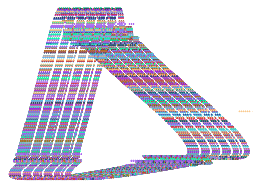
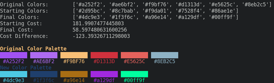
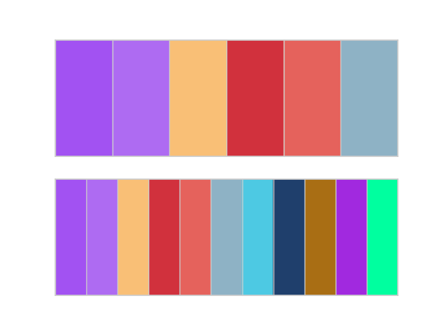
I used the color palette generator to set the colors for this blog. Here is the output:
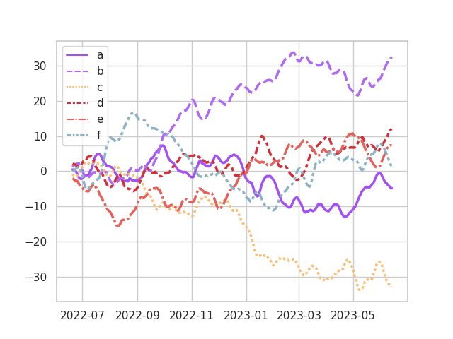
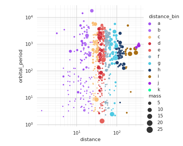
Some Plots
Original Palette
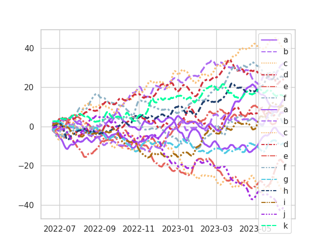
Extended Palette
Comparison of Palettes
Original Palette
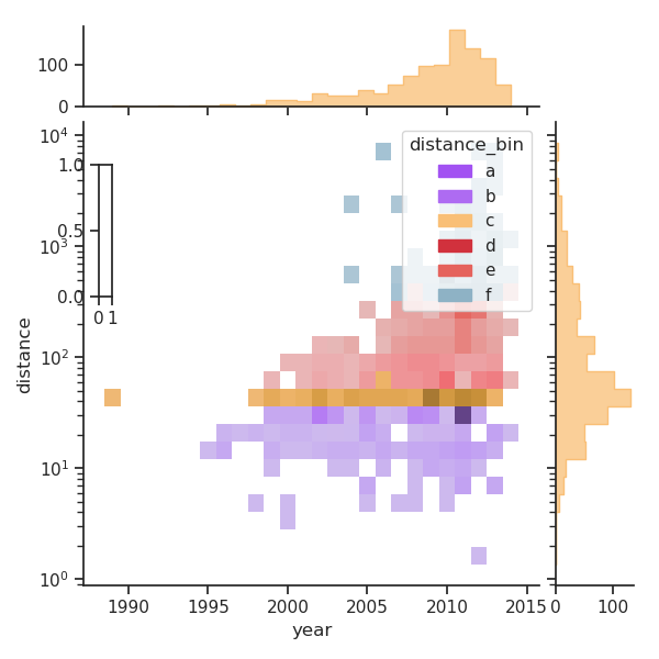
Extended Palette
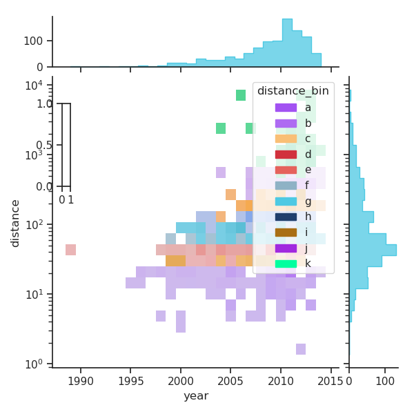
Original Palette
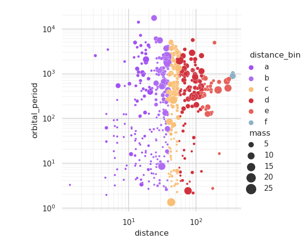
Extended Palette
The Code
Color
See the whole file here
There are 2 major pieces for the color module: the Color object and the average_color_distances_from_target function
class Color:
    def __init__(self, red: float, green: float, blue: float):
        """
        Represents a color. Provides functionality for using both RGB values in [0, 255]
        or a hex as an initializer.
        For hex initialization, use Color.from_hex("#your_hex_value")
        Args:
            red: A float in [0, 255] representing the amount of red in the color
            green: A float in [0, 255] representing the amount of green in the color
            blue: A float in [0, 255] representing the amount of blue in the color
        """
        self.rgb = np.array([red, green, blue])
        self.rgb = np.array([clip_values(val) for val in [red, green, blue]])
        self.hex = self.to_hex()
        self.lab_color = convert_color(sRGBColor(*self.rgb), LabColor)

    @classmethod
    def from_hex(cls, hex_value: str) -> Color:
        """
        Initialize a color object using a hex value
        Args:
             hex_value: A string containing a hex value, e.g. '#ffffff'
        Returns:
            A Color object for the given color
        """
        rgb = np.array(matplotlib.colors.to_rgb(hex_value)) * 255
        return Color(*rgb)

    @classmethod
    def random_color(cls) -> Color:
        """
        A classmethod that returns a random color
        Usage:
             > Color.random_color()
        """
        rgb = np.random.choice(range(1, 256), 3)
        return Color(*rgb)

    def to_hex(self) -> str:
        """
        returns a hex value for the given RGB value
        """
        return matplotlib.colors.to_hex(self.rgb / 255)

    def delta_e(self, other_color: Color) -> float:
        """
        Returns the ΔE value for the distance between 2 colors. Uses the CIEDE2000 definition
        Args:
            other_color: Another color object to compare against
        Returns:
            A float showing the 'distance' between the colors
        Notes:
            > https://en.wikipedia.org/wiki/Color_difference#CIEDE2000
        """
        return delta_e_cie2000(self.lab_color, other_color.lab_color)

    def get_closest_color(self, color_list: List[Color]) -> Tuple[Color, float]:
        """
        Given a color list, get the color which is closest to the Color object calling this method via ΔE.
        Args:
            color_list: A list of Color objects to compare
        Returns:
             A tuple containing the closest color's Color object and the ΔE value
        """
        distances = [self.delta_e(other_color) for other_color in color_list]
        min_val = np.argmin(distances)
        return color_list[min_val], distances[min_val]

    def nearby_color(self, drift_control: float = 0.1) -> Color:
        """
        Returns a 'nearby' color. Essentially takes a color, chooses a value in [R, G, B]
        and adds some random drift to it
        Args:
            drift_control: How much to allow randomness to affect the value update
        Returns:
            Returns a new Color object that is slightly different from the current color
        """
        index = np.random.choice(range(3), 1)
        new_rgb = self.rgb.copy()
        new_val = (new_rgb[index] / 255.) + np.random.rand() * drift_control - 0.05

        if new_val > 1:
            new_val = 1
        elif new_val < 0:
            new_val = 0

        new_rgb[index] = new_val * 255

        return Color(*new_rgb)
In the Color object, there are 3 really important methods:
delta_e
This returns the delta E color measure. It is essentially the distance of 2 colors from each other. Here is a better definition from Wikipedia:
The difference or distance between two colors is a metric of interest in color science. It allows quantified examination of a notion that formerly could only be described with adjectives. Quantification of these properties is of great importance to those whose work is color-critical. Common definitions make use of the Euclidean distance in a device-independent color space.
Nice. I didn't know this existed before!
get_closest_color
Given a list, this returns the color that is closest to it. This is used in the averagecolordistancesfromtarget function below to get the average distance between the colors passed to the function and the target colors you are seeking to get closer to.
def average_color_distances_from_target(color_list: List[Color], target_colors: List[Color]) -> float:
    """
    Given 2 color lists, get the average distance between the colors
    Args:
        color_list: the input color list
        target_colors: the color list to compare it to. These arguments have arbitrary order
    Returns:
        The average distance value (ΔE)
    """
    distances = list(map(lambda c: c.get_closest_color(target_colors)[1], color_list))
    return np.average(distances)
nearby_color
Usually, with hill-climbing algorithms, you need some way to perturb the state space to test if the change is a good thing or not. In this program, nearby_color is how it is done. The idea here is to change the color very slightly. Then we can compare our new color to the set of colors we are optimizing toward and if it is a step in the right direction, it will stick with some probability.
The algorithm is the following:
- Start with a channel value for red, green, and blue: \([R, G, B]\)
- Randomly select a channel
- Normalize the value (it starts in \([0, 255]\)) and then add a uniform random variable to it
- in this case, I also added a fun named variable drift control which allows you to bound how much change the uniform R.V. can affect the step size of the algorithm. If you crank this up, your step size gets larger, leading to more movement in the color space each time the nearbycolor method is called
- Clip the value so it is in \([0, 1]\)
- Multiply by 255 to return to \([0, 255]\) space
Brettel
See the whole file here
The core piece of the brettel module is the Brettel class. This is the class that adjusts for color blindness
class Brettel:

    BRETTEL_PARAMS = {
        'protan': {
            'rgb_cvd_from_rgb1': [0.1451, 1.20165, -0.34675, 0.10447, 0.85316, 0.04237, 0.00429, -0.00603, 1.00174],
            'rgb_cvd_from_rgb2': [0.14115, 1.16782, -0.30897, 0.10495, 0.8573, 0.03776, 0.00431, -0.00586, 1.00155],
            'separation_plane_normal': [0.00048, 0.00416, -0.00464]},
        'deutan': {
            'rgb_cvd_from_rgb1': [0.36198, 0.86755, -0.22953, 0.26099, 0.64512, 0.09389, -0.01975, 0.02686, 0.99289],
            'rgb_cvd_from_rgb2': [0.37009, 0.8854, -0.25549, 0.25767, 0.63782, 0.10451, -0.0195, 0.02741, 0.99209],
            'separation_plane_normal': [-0.00293, -0.00645, 0.00938]
            },
        'tritan': {
            'rgb_cvd_from_rgb1': [1.01354, 0.14268, -0.15622, -0.01181, 0.87561, 0.13619, 0.07707,0.81208, 0.11085],
            'rgb_cvd_from_rgb2': [0.93337, 0.19999, -0.13336, 0.05809, 0.82565, 0.11626, -0.37923, 1.13825, 0.24098],
            'separation_plane_normal': [0.0396, -0.02831, -0.01129]
            },
        }

    def __init__(self, sRGB: List[float]):
        """
        Changes sRGB ranges to account for color blindness types and severity
        Usage:
            Access the various functions through their attributes. For example:
            > Brettel(sRGB_value).Deuteranomaly
        Args:
            sRGB: A list of floats representing a color in sRGB format [R, G, B]
        """
        self.Normal = sRGB
        self.Protanopia = self.brettel(sRGB, 'protan', 1.0)
        self.Protanomaly = self.brettel(sRGB, 'protan', 0.6)
        self.Deuteranopia = self.brettel(sRGB, 'deutan', 1.0)
        self.Deuteranomaly = self.brettel(sRGB, 'deutan', 0.6)
        self.Tritanopia = self.brettel(sRGB, 'tritan', 1.0)
        self.Tritanomaly = self.brettel(sRGB, 'tritan', 0.6)
        self.Achromatopsia = monochrome_with_severity(sRGB, 1.0)
        self.Achromatomaly = monochrome_with_severity(sRGB, 0.6)

    def brettel(self, sRGB: List[float], cb_type: str, severity: float) -> List[float]:
        """
        Brettel adjustment to a given color
        Args:
            sRGB: A list of [R, G, B] values comprising a color
            cb_type: color blindness type to account for
            severity: the severity of the color blindness to account for
        Returns:
            A list of floats in sRGB space transformed to account for the color blindness type in [0, 255] space
        Notes:
            > http://vision.psychol.cam.ac.uk/jdmollon/papers/Dichromatsimulation.pdf
        """
        rgb = [sRGB_to_lRGB(v) for v in sRGB]
        params = Brettel.BRETTEL_PARAMS[cb_type]
        separation_plane_normal = params['separation_plane_normal']

        # check on which plane we should project by comparaing with the separation plane normal
        sep_plane_dot = np.dot(rgb, separation_plane_normal)
        rgb_cvd_from_rgb = params['rgb_cvd_from_rgb1'] if sep_plane_dot >= 0 else params['rgb_cvd_from_rgb2']

        # transform to the full dichromat projection plane
        rgb_cvd = [np.dot(rgb_cvd_from_rgb[:3], rgb),
                   np.dot(rgb_cvd_from_rgb[3:6], rgb),
                   np.dot(rgb_cvd_from_rgb[6:9], rgb)]

        # apply the severity factor as a linear interpolation
        rgb_cvd[0] = rgb_cvd[0] * severity + rgb[0] * (1.0 - severity);
        rgb_cvd[1] = rgb_cvd[1] * severity + rgb[1] * (1.0 - severity);
        rgb_cvd[2] = rgb_cvd[2] * severity + rgb[2] * (1.0 - severity);

        # return sRGB values
        return [lRGB_to_sRGB(v) for v in rgb_cvd]
This code was essentially taken from: brettel colorblind simulation which is a part of the jsColorBlindSimulator project. What it does is take an RGB value and transform it so that it works well for people with the given type of color blindness.
All those constants at the top of the class are an approximation of the weights that would be used for the transformation. The rest of the class is the actual transformation method brettel and a bunch of attributes that allow for different method calls.
The optimization algorithm gives lower weight to the color blindness parameters than it does to get close to the original palette. Having the adjustment for color blindness is nice though since by accounting for the different ways in which people perceive color differences, our algorithm tends to optimize for slightly higher contrast overall.
If you want to dig into the underlying principles of Brettel et. al's work, check out the paper
Annealing (Optimization)
See the whole file here with all of the helper functions and constants
There are 2 main pieces to the optimization module: the objective function obj_fn and the optimization step anneal.
def obj_fn(state: List[Color], target_colors: List[Color]) -> float:
    """
    An objective function that measures the distance between the current state (list of colors)
    and the target state (target_colors). Tweak the weights to change the output.
    From the original documentation:
    A higher
        > normal weight will result in colors that are more differentiable from each other
        > range weight will result in colors that are more uniformly spread through color space
        > target weight will result in colors that are closer to the target colors specified with targetColors
        > protanopia weight will result in colors that are more differentiable to people with protanopia
        > deuteranopia weight will result in colors that are more differentiable to people with deuteranopia
        > tritanopia weight will result in colors that are more differentiable to people with tritanopia
    Args:
        state: A list of colors representing the current iteration of the state of your optimization function
        target_colors: A list of colors representing the goal to work towards for your optimization function
    Returns:
        A float representing the 'score' of the current state
    """
    weights = {'Normal': 1,
               'Range': 1,
               'Target': 1,
               'Protanopia': 0.33,
               'Deuteranopia': 0.33,
               'Tritanopia': 0.33}

    # get distances of state from target w.r.t each of the different color blindness measures
    distances = {n: corrected_color_distances(state, n)
                 for n in ['Normal', 'Protanopia', 'Deuteranopia', 'Tritanopia']}

    # generate the 'scores'
    scores = merge(
        {n: 100 - np.average(distances[n])
         for n in ['Normal', 'Protanopia', 'Deuteranopia', 'Tritanopia']},
        {'Range': np.max(distances['Normal']) - np.min(distances['Normal']),
         'Target': average_color_distances_from_target(state, target_colors)})

    return (weights['Normal'] * scores['Normal'] +
            weights['Target'] * scores['Target'] +
            weights['Range'] * scores['Range'] +
            weights['Protanopia'] * scores['Protanopia'] +
            weights['Deuteranopia'] * scores['Deuteranopia'] +
            weights['Tritanopia'] * scores['Tritanopia'])
The custom objective function is where the magic happens.
It assigns weights to our different considerations (various types of color blindness and "Normal" which is the unfiltered measure). Then it runs the color blindness transformations and measures the average distance (using delta E) between the set of colors that are given to the function and our target palette. From there we create a score and then sum up the dot product of the weights and scores.
This score is a rough measure of how close to our goal we are. Since it is an approximation, it is exceedingly unlikely that it will go to 0 (but will approach 0 until it stalls out).
def anneal(input_colors: List[Color], result_count: int = 5,
           temperature: float = 1000., cooling_rate: float = 0.99, cutoff: float = .0001,
           objective_function: Callable = obj_fn,
           verbose: bool = True) -> List[Color]:
    """
    A simulated annealing hill climbing algorithm that attempts to minimize the distance from
    the input colors and random set of colors as measured by the objective_function
    Args:
        input_colors: A list of target colors to optimize toward
        result_count: How many colors to return
        temperature:  starting point temperature of the algorithm; higher temperature means that
                      early iterations are more likely to be randomly-chosen than optimized.
        cooling_rate: decrease in temperature at each iteration. A lower cooling rate will result in more iterations.
        cutoff:       temperature at which the algorithm will stop optimizing and return results
        objective_function: the objective function with which to measure success. Defaults to obj_fn
                            requires a target_colors parameter to accept the goal state
        verbose: print out the current temperature and cost?
                 Also prints out the (target, starting, final) color lists and (starting, final, difference) costs
    Side Effect:
        If verbose, prints to the console
    Returns:
        A list of the final resulting colors (in Color objects)
    """
    # get a random set of initial colors
    colors = [Color.random_color() for _ in range(result_count)]

    # set the objective function
    obj_fn = curry(objective_function, target_colors=input_colors)

    start_colors = colors.copy()
    start_cost = obj_fn(colors)

    while temperature > cutoff:
        for i in range(len(colors)):
            # copy colors
            new_colors = colors.copy()
            # move the current color randomly
            new_colors[i] = new_colors[i].nearby_color()
            # get objective function difference
            delta = obj_fn(new_colors) - obj_fn(colors)
            # choose between current and new state
            probability = np.exp(-delta / temperature)
            if np.random.rand() < probability:
                colors[i] = new_colors[i]

        if verbose:
            print(f"current cost:\t\t{obj_fn(colors)}")
            print(f"current temperature:\t{temperature}")

        temperature *= cooling_rate

    final_cost = obj_fn(colors)

    if verbose:
        print(dedent(f"""
                      Original Colors:\t{hex_list(input_colors)}
                      Starting Colors:\t{hex_list(start_colors)}
                      Final Colors:\t\t{hex_list(colors)}
                      Starting Cost:\t\t{start_cost}
                      Final Cost:\t\t{final_cost}
                      Cost Difference:\t{final_cost - start_cost}
                      """))

    return colors
The optimization function is using Simulated Annealing
Here is the pseudocode for simulated annealing for comparison:
- Let \(s = s_0\)
- For \(k = 0\) to \(k_{max}(\mathrm{exclusive})\):
- T = temperature(\(1 - (k + 1) / k_{max}\))
- Pick a random neighbor \(s_{new}\) = neighbor(s)
- If \(P(E(s), E(s_{new}), T) \geq\) random(0, 1):
- \(s\) = \(s_{new}\)
- Output the final state \(s\)
We can see this maps particularly well to the code:
- Let colors = (random assortment of colors) # starting state
- For each color in colors:
- T = temperature(given color)
- Pick a random nearby color
- measure the difference between the new set of colors and our target colors (using the objective function) \(\Delta\)
- check if the probability of acceptance \(P\) is greater than a random number in [0, 1] where \(P\) is a function of our \(\Delta\) and our temperature T
- if so, keep it!
- Lower the temperature a bit and iterate
- Output the final set of colors
- \(P\) is the commonly used heuristic function \(P = e^{-\frac{\Delta}{T}}\)
Possible Enhancements
- encode all the colors into numerical space and only use vectorized numpy operations
- Update the simulated annealing algorithm
- better yet, find an optimization engine that allows a simpler formulation of the goal and a more battle-tested package (maybe scipy.optimize)
- Try to find an ideal weighting of the different aspects for different goals. Maybe create a series of pre-made settings that focus on different use-cases.
- Instead of trying to make complementary palettes, try making palettes that are very different
- Possibly change the weights of the Brettel class?
- From the jsColorBlindSimulator project:
The Brettel, Viénot and Mollon Simulation function This is an implementation of the research paper Computerized simulation of color appearance for dichromats by Brettel, H., Viénot, F., & Mollon, J. D. (1997). It has been adapted to modern sRGB monitors and should be pretty accurate, at least for full dichromacy. Of course, it is still an approximation though, many factors make it imperfect, such as an uncalibrated monitor, unknown lighting environment, and per-individual variations. In general, it will tend to be accurate for small or thin objects (small dots, lines) and too strong for large bright areas, even for full dichromats.
Maybe something that adjusts the levels of the Brettel transformation given the context in which the palette will be used? It could be useful to tone it down if you are making art with large swaths of consistent color
Possible Future Projects
Some things I think would be neat to build using this:
- The aforementioned emacs theme generator
- A package that dynamically generates and caches a theme for you whenever you plot some data with more categorical variables than your given theme supports
- A stylesheet generator that allows the end-user of a website many options for theming the website they are viewing
- Palettes for generative art
- A placeholder image/thumbnail generator that conforms to a color palette for WIP websites
- Palettes for light shows and visualizers
If you find any of these interesting, please reach out! (email in about page)