Searching For Chaos
Attention Conservation Notice
An attempt to find pretty bits of art by playing with coefficients on a 2D system of nonlinear differential equations (2D Quadratic Maps based on the Hénon map). Exploring this in sufficient depth would lead to a lot of fun in chaos theory / nonlinear dynamics-land. This is not sufficient depth
The Generative Art Internet
What a wonderful place! People all over the world tinker with math and scripts to make beautiful art. I was looking at old blog posts from Fronkonstin and thought it would be fun to recreate the Chaotic Galaxies post and tinker with the code.
Fronkonstin was nice enough to link where he found the initial content:
Strange Attractors: Creating Patterns in Chaos
The author (Julien Sprott) was gracious and provided the book for free on his website. All of the code from the book is in some dialect of BASIC. The content in the book is a fun read; it provides an exciting build-up of strange attractors and nonlinear dynamics, starting from the simplest 1D maps. I haven't read it all, but from what I have read he brings the content to life without assuming that you are a graduate student in analysis.
Recreation
My first goal is to recreate the plots that Fronkonstin made
Differential Equations
The system of differential equation that this post hinges on is the following:
The Code
The code looks super simple on Fronkonstin's blog. It consists of the differential equation function definitions, a set of coefficients, a function that generates the steps iteratively, and a plotter. These pieces map to python well
The Equations
The Coefficients
The function that generates the steps iteratively
the plotter
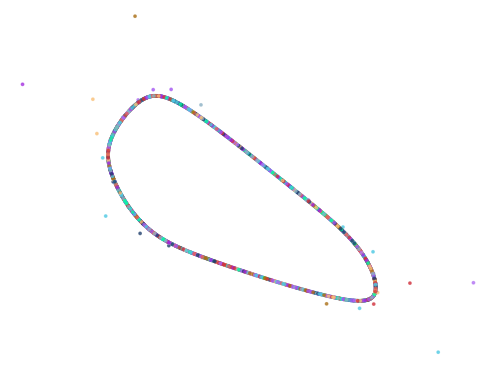
Now we have all the pieces, and can generate some plots!
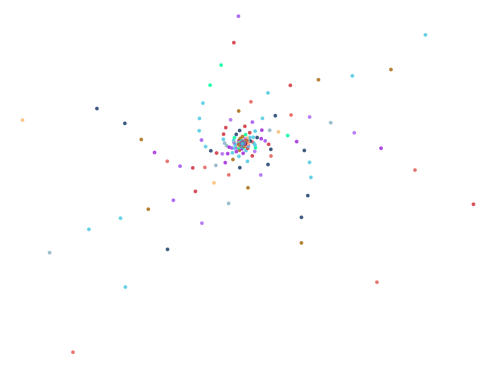
Initial Curated Plots
Z1 Coefficients: [1.0, -0.1, -0.2, 1.0, 0.3, 0.6, 0.0, 0.2, -0.6, -0.4, -0.6, 0.6]
Z2 Coefficients: [-1.1, -1.0, 0.4, -1.2, -0.7, 0.0, -0.7, 0.9, 0.3, 1.1, -0.2, 0.4]
Z3 Coefficients: [-0.3, 0.7, 0.7, 0.6, 0.0, -1.1, 0.2, -0.6, -0.1, -0.1, 0.4, -0.7]
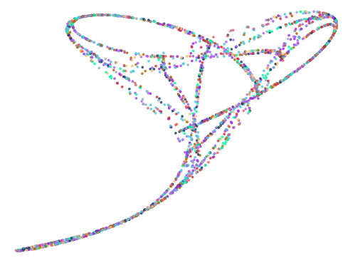
Z4 Coefficients: [-1.2, -0.6, -0.5, 0.1, -0.7, 0.2, -0.9, 0.9, 0.1, -0.3, -0.9, 0.3]
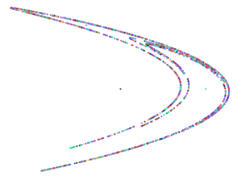
Z5 Coefficients: [1.0, 0, -1.4, 0, 0.3, 0, 0, 1, 0, 0, 0, 0]
Z5 is the Hénon map, a special case of our more general map.
After generating the plots on the blog, I hoped to begin tweaking the coefficients and generating some new pictures.
Fronkenstin gives the words of encouragement:
Changing the vector of parameters you can obtain other galaxies. Do you want to try?
Initial Attempts at State Space Search
Chaotic systems must have these properties:
- it must be sensitive to initial conditions
- it must be topologically transitive
- it must have dense periodic orbits
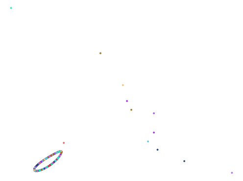
The idea was to tweak initial parameters and get some cool plots. Unfortunately, just choosing random initial parameters is not guaranteed to give us an interesting output. Only a small subset of the possible sets of coefficients will give us an interesting strange attractor output. Most of the sets of coefficients will either blow up to , or return nothing interesting at all.
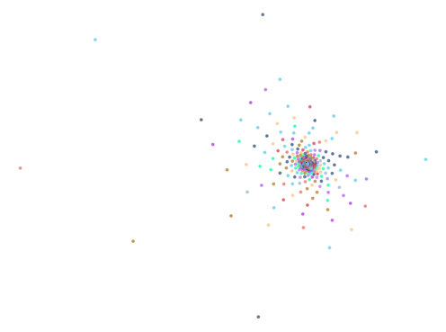
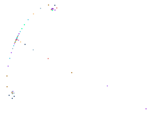
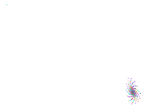
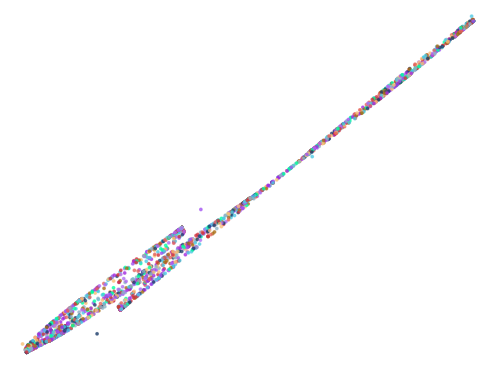
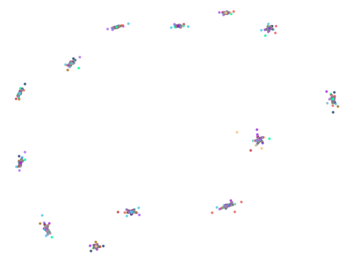
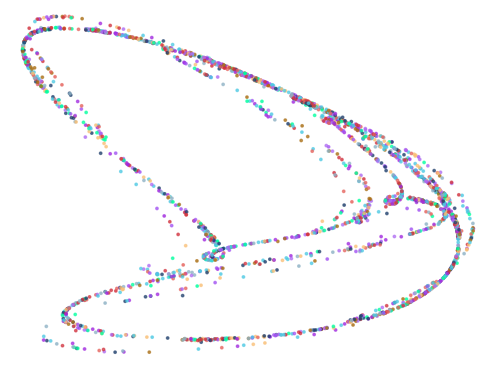
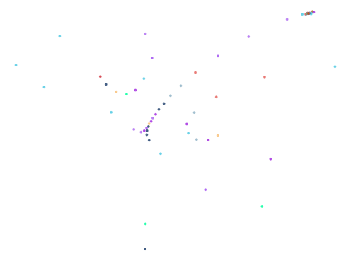
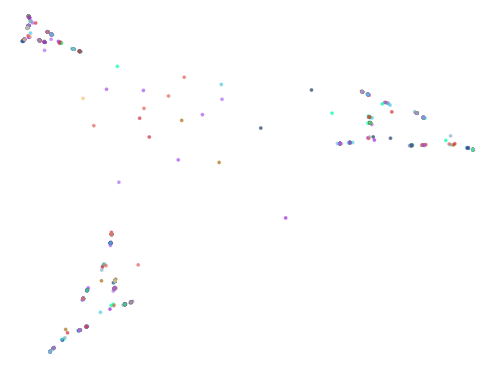
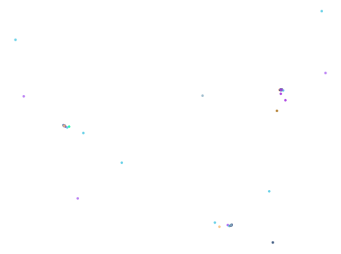
I tried out some random sets of the 12 coefficients in the hopes that I would find something, but that was inefficient and returned mostly garbage. The overwhelming majority of images were just random splashes of color on a dark background.
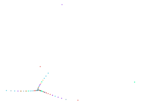
Here are some examples of the majority of plots produced:
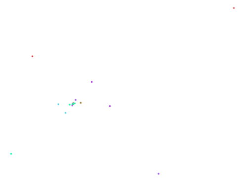
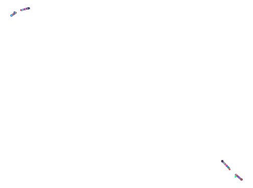
Not too thrilling!
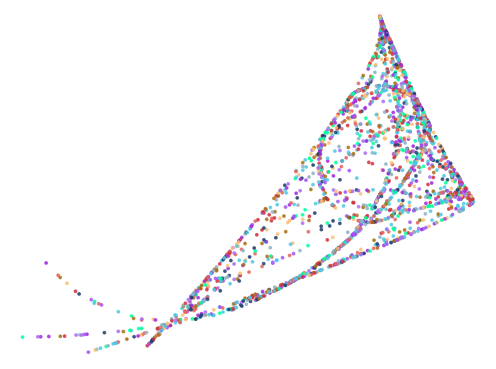
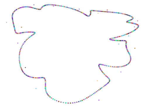
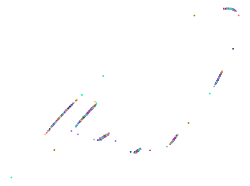
After a while of tinkering, I ended up constraining the space in which I generated the coefficients and got some better results:
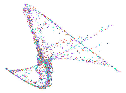
Here is the script for generating the more interesting outputs:
You can tweak the values that lies in to get different outcomes.
Most of the results look like the underwhelming sparse dots of color on a dark background. Out of 10,000 iterations, the algorithm above yielded 70 results that fit the criteria and didn't result in an overflow error.
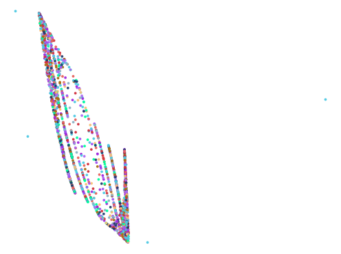
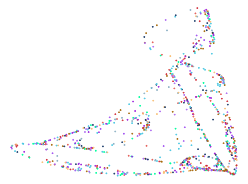
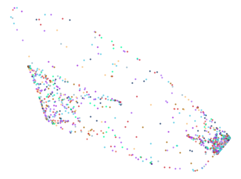
Of those 70 results, only a handful looked interesting.
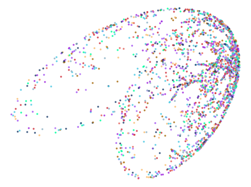
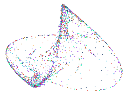
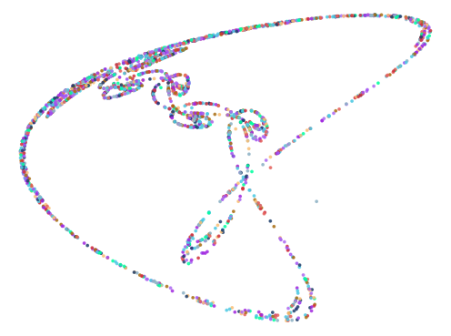
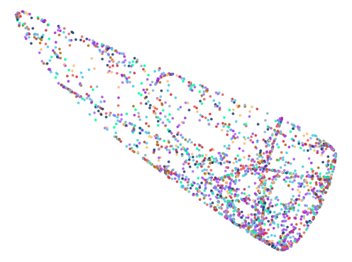
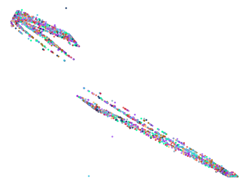
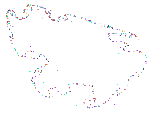
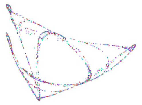
Here are some of the more interesting ones:
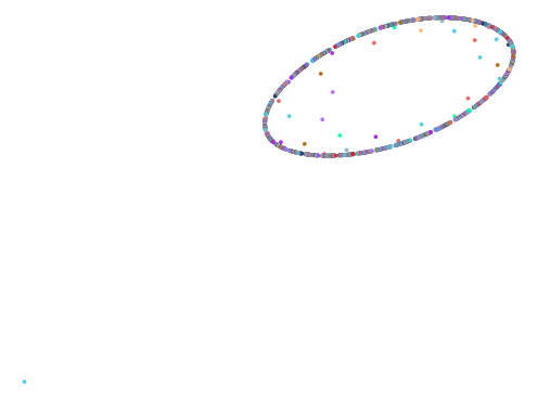

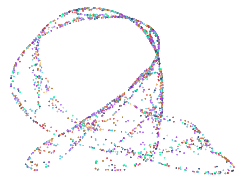
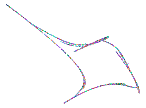
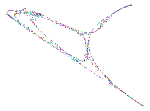
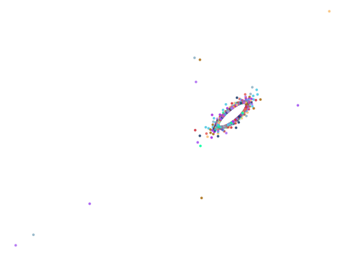
The next batch was ran with 0.75 < abs(a - b) < 1.5
Of the 10,000 iterations, the algorithm found 451 results.
How were the effective coefficients found by others?
It seems that there is an island of instability for these types of maps. Here is a view of state space for the simple Hénon map:
From the book:
As with the logistic map, the Hénon map has unbounded solutions, chaotic solutions, and bounded nonchaotic solutions, depending on the values of a and b. The bounded nonchaotic solutions may be either fixed points or periodic limit cycles. Figure 8-1 shows a region of the ab plane with the four classes of solutions indicated by different shades of gray.
The bounded solutions constitute an island in the ab plane. On the northwest shore of this island is a chaotic beach, which occupies about 6% of the area of the island. The chaotic beach has many small embedded periodic ponds. The boundary between the chaotic and the periodic regions is itself a fractal.
There is also more information on these boundaries here
Like all bouts of tinkering, I need to read some source material if I want to get better results! Thankfully, the book is available for free on the author's website!
The Book & Encoding
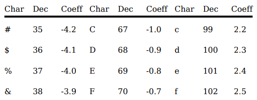
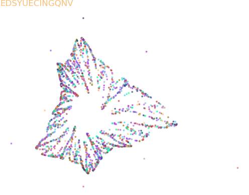
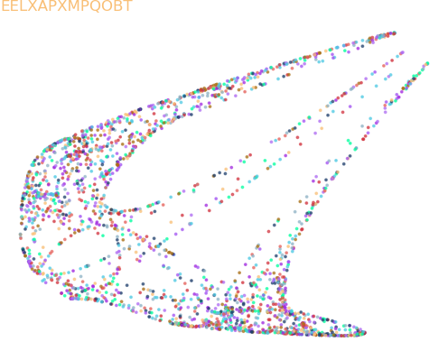
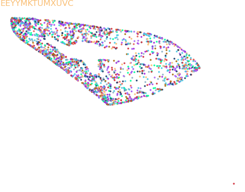
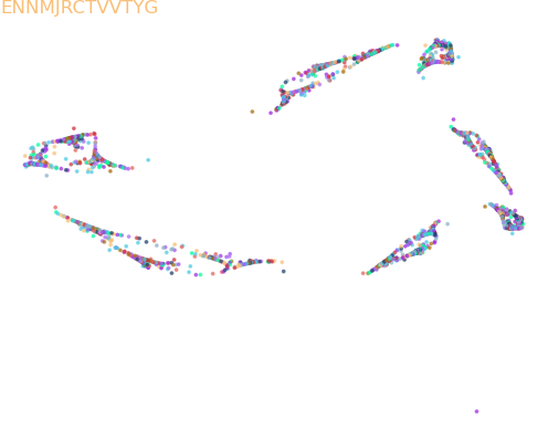
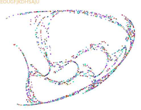
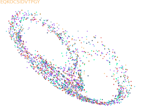
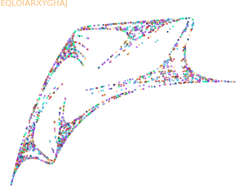
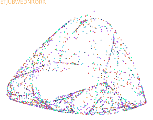
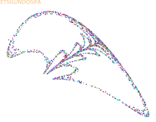
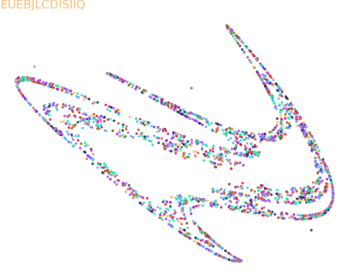
In the book, the author uses a coding system to represent different coefficient values. It looks like this:
Then he outputs the key at the top of each plot:
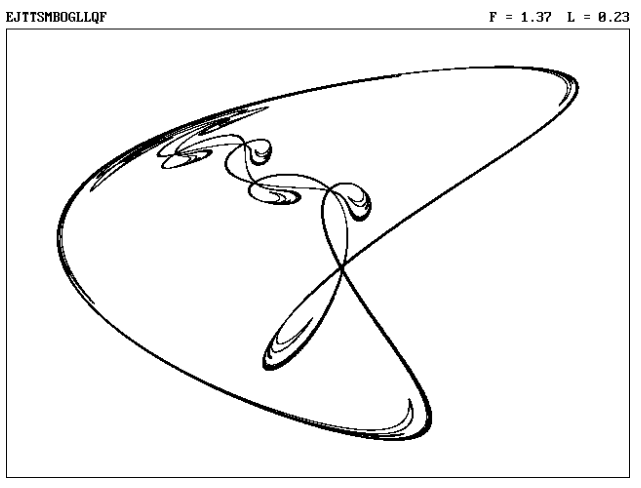
In this case, he leads with an E as a code for a quadratic 2-dimensional map and the rest of the letters translate to coefficients in the key.
For example, J = -0.3, T = 0.7, S = 0.6, M = 0.0, B = -1.1, and so on until you have all 12 coefficients for this map. This becomes handy further in the book as the degree of the polynomials increases (and allows for even more complexity of output).
If I do a follow-up post, this method could be used to make more intricate strange attractors (with higher degree polynomials)
Unfortunately, random choosing these values doesn't seem to be super helpful (we tried that above), but it does allow us to recreate some of the nice figures from the book with a simple codename:
additional plots
Searching For More
It would be helpful if we had a way to directly determine if a given set of coefficients leads to a chaotic output without viewing the plots.
It seems this is a difficult problem: How to know whether an Ordinary Differential Equation is Chaotic?
Makeshift Measures of Chaotic Bulbousness
What a neat title! That could be a band name.
What I want is to find a way to consistently generate bulbous (roundish, relatively self-contained) strange attractors.
How do we measure the bulbousness of a strange attractor?
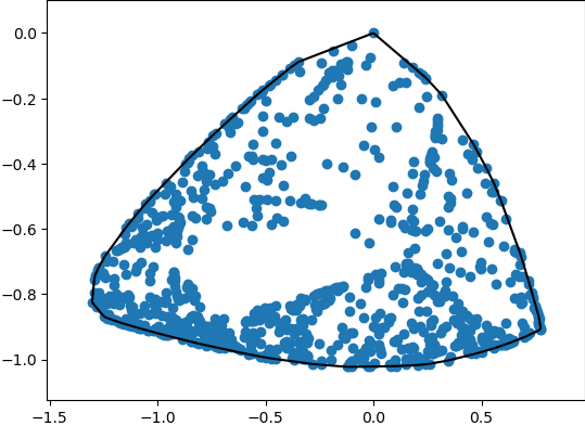
The idea:
- generate a convex hull around the strange attractor
-
figure out how many clusters there are in the data. This is akin to cross-validation for a clustering algorithm.
-
divide the area of the convex hull by the number of cluster groups
bulbous = convex hull area / k groups
!!! Note that in 2 dimensions, ConvexHull volume attribute is actually area
For our results, we want something that is mostly contained in a single group (or a couple of groups) and has a relatively large area. We seek to maximize our bulbous area.
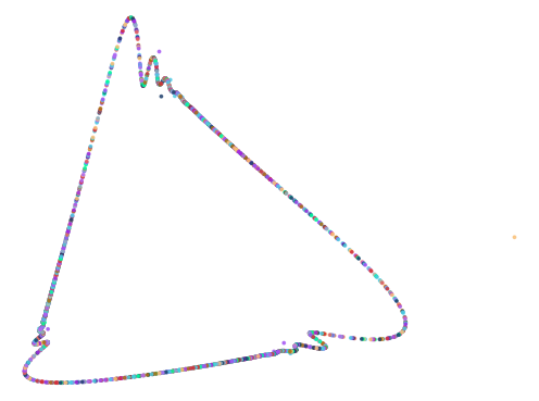
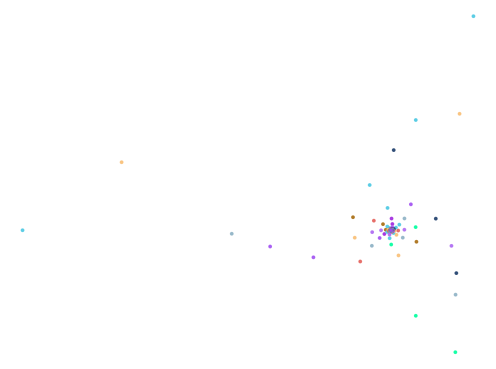
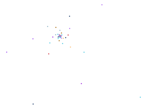
Of the 10,000 iterations, the algorithm found 12 results
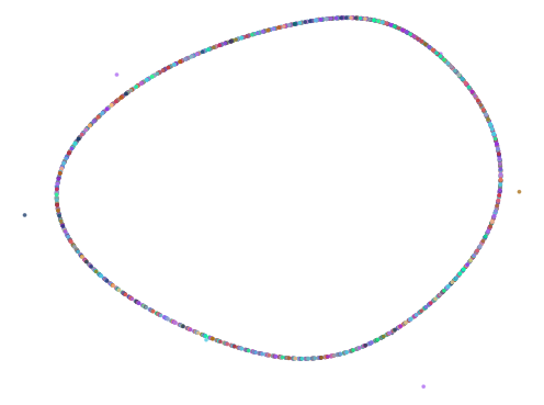
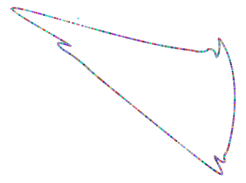
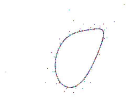
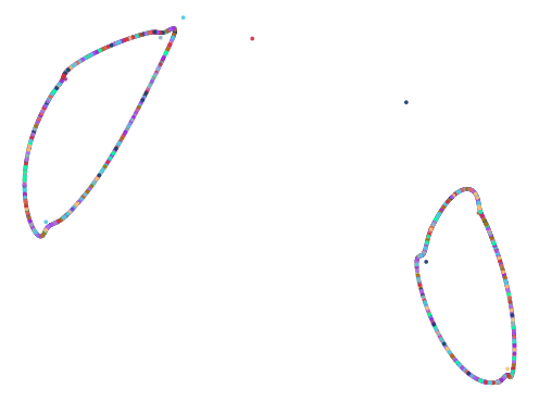
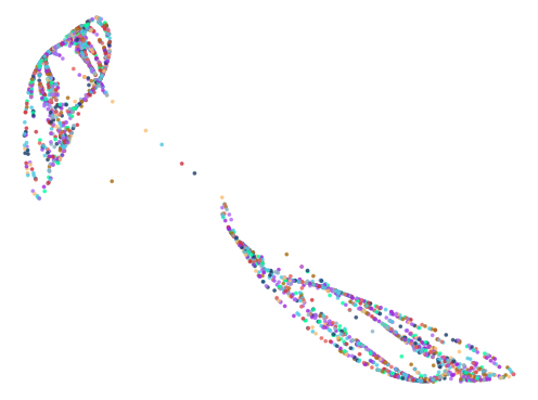
Bulbous Measure Plots
Did it work? kind of. Here are the plots in descending order of the bulbous measure:
Enhancement Ideas
-
Find a way to get rid of outliers so that the numerator (area) isn't large for very diffuse images
- Use the optimal K algorithm above to fit a Gaussian Mixture Model and then eradicate values that are far from the centers
- Fit a linear model and use Cook's Distance to remove points that give a lot of pull
- Use an anomaly detection algorithm like Isolation Forest to remove outliers
-
Some kind of variance/concentration measure
-
We could check for cycles and once we find one (if we find one) we can take the average pairwise distance between each point (assuming the set of points in a cycle is manageable). Then we could remove those points that have average distances greater than some cutoff.
-
Throw a neural network at it
- Label a dataset of images that are appealing to the eye along with their coefficient sets
([coefficient_1, ..., coefficient_n], appealing_binary_indicator)- Train a network to predict (for a given set of coefficients) whether it would lead to an appealing image