A few weeks ago I picked up the TidyTuesday 2025 Week 3 dataset on Himalayan mountaineering expeditions. The data comes from the Himalayan Database, a remarkable archive maintained by Elizabeth Hawley and her successors since 1963.

This is the first post in a series on Himalayan mountaineering data. Here I'll introduce the dataset and talk about why I found it interesting. The next post covers exploratory data analysis.

Why This Dataset?

I was drawn to this data for a few reasons:

It has natural hierarchical structure. Expeditions are nested within peaks. Peaks are nested within regions. Members are nested within expeditions. This kind of structure is everywhere—students within schools, patients within hospitals, trades within portfolios—and the modeling patterns transfer.

The outcome is binary with rare events. Summit success is 0/1. Deaths are rare but consequential. Both of these create interesting modeling challenges: imbalanced classes, small samples per group, the need for shrinkage estimators.

Confounding is obvious. Oxygen use is strongly associated with success—but expeditions that use oxygen also tend to be on higher peaks, with more resources, in commercial settings. The naive association is not the causal effect. This makes it a good teaching example for causal reasoning.

The domain is tangible. Unlike financial data or abstract simulations, mountaineering has a visceral quality. The 8,000-meter "Death Zone" isn't a metaphor—it's where human physiology breaks down and success rates plummet.

The Data at a Glance

Two main tables:

The expeditions table contains the outcome variables I care about:

• success1/success2: Binary indicators for whether anyone summited
• mdeaths/hdeaths: Member and hired staff deaths
• o2used: Whether supplemental oxygen was used
• totmembers/tothired: Team composition

The peaks table provides context:

• heightm: Peak height in meters
• pyear: Year of first ascent
• pkname: Peak name (Everest, Cho Oyu, etc.)

These join on peakid, which is the key for hierarchical modeling.

The Nested Structure

Here's the conceptual model:

Region → Peak → Expedition → Outcome
         ↓
       Height
       First Ascent Year
       Historical Success Rate

Each level adds information:

• Regions have different weather patterns and accessibility
• Peaks have intrinsic difficulty (height, technical routes)
• Expeditions have team composition, timing, resources
• Outcomes are the success/failure we're trying to predict

This is the structure that hierarchical models are designed for. A standard logistic regression treats all expeditions as independent; a multilevel model recognizes that expeditions on the same peak share unobserved characteristics.

The practical implication: when a peak has only 3 expeditions (all successful), should we believe its "100% success rate"? Probably not—that's sampling variability. Hierarchical models shrink these extreme estimates toward the overall mean, which is exactly what Empirical Bayes does. More on this in the third post.

Key Variables for Modeling

After exploring the data, these emerged as the primary predictors:

Peak Height (The Big One)

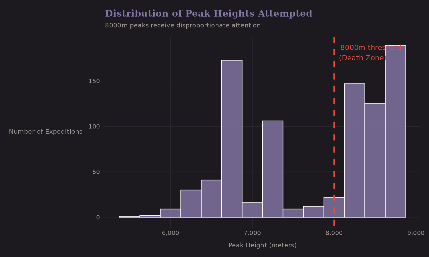
The 8,000-meter threshold isn't arbitrary—it marks the "Death Zone" where supplemental oxygen becomes nearly essential. Above this altitude:

• The partial pressure of oxygen is ~1/3 of sea level
• Most climbers can survive only 2-3 days without supplemental O2
• Success rates without oxygen drop dramatically (~14% at 8000m+ vs ~72% below 7000m)
• Death rates spike

Here's the twist: the overall success rate at 8000m+ is actually the highest (~76%) because nearly all expeditions there use supplemental oxygen (~82%), and with oxygen, success rates reach ~89%. This is a classic example of Simpson's Paradox—the conditional relationship (higher = harder) reverses when you aggregate across oxygen use.

Season

Spring (pre-monsoon) dominates Himalayan climbing. The jet stream lifts off the peaks briefly, creating weather windows. Autumn is the secondary season. Summer and winter attempts are rare and riskier.

Team Composition

Solo attempts behave differently from team expeditions. The ratio of hired staff (Sherpas, porters) to members captures resource investment. Higher staff ratios are associated with better outcomes—but again, this is confounded with commercial expeditions on popular routes.

Supplemental Oxygen

The naive correlation between oxygen use and success is huge. But interpreting this causally requires care. Expeditions don't randomly choose whether to use oxygen—the choice is correlated with:

• Peak height (nearly universal above 8,000m)
• Commercial vs. alpine style
• Team resources
• Risk tolerance

A proper causal analysis would need matching, instrumental variables, or careful conditioning. I don't attempt that here, but I flag it as a trap.

Thinking in Hierarchies

One of the transferable skills from this analysis is thinking in hierarchies.

In my day job (private equity), we often encounter nested data:

• Companies within funds within firms
• Quarters within years within economic cycles
• Deals within sectors within vintages

The same modeling patterns apply. A fund's track record with 5 deals tells us something, but not as much as the track record of a firm with 50 deals across 10 funds. Shrinkage estimators help us weight appropriately.

In machine learning, hierarchical thinking shows up as:

• Transfer learning (leverage related tasks)
• Grouped cross-validation (don't leak within groups)
• Mixed effects in survival analysis

The Himalaya data is a nice pedagogical example because the hierarchy is concrete. You can see why Everest expeditions are different from Ama Dablam expeditions, even if both are "Himalayan mountaineering."

What's Next

The next post digs into exploratory analysis: missing data patterns, temporal trends, and the correlation structure among predictors.

If you want to follow along, the data is available from the TidyTuesday repo:

library(tidyverse)

exped <- read_csv(
  "https://raw.githubusercontent.com/rfordatascience/tidytuesday/main/data/2025/2025-01-21/exped_tidy.csv"
)

peaks <- read_csv(
  "https://raw.githubusercontent.com/rfordatascience/tidytuesday/main/data/2025/2025-01-21/peaks_tidy.csv"
)

Or use the tidytuesdayR package to load it directly.