Probabilistic Graphical Models
This is the fifth post in a series on Himalayan mountaineering data. The previous post covered Bayesian hierarchical models. Here I'll explore Probabilistic Graphical Models—a framework for encoding causal assumptions and reasoning about conditional independence.
PGMs are powerful because they make assumptions explicit. Instead of implicitly conditioning on confounders, we draw the causal structure and let the math tell us what needs to be controlled.
What's a PGM?
A Probabilistic Graphical Model represents a joint probability distribution using a graph. Nodes are random variables; edges encode dependencies.
Directed graphs (DAGs) show causal direction. An arrow A → B means "A causes B" (or at least, A is a potential cause). The absence of an arrow means no direct causal effect.
Bayesian networks are DAGs with conditional probability tables. Given the graph structure, we can compute P(any variable | evidence) using message-passing algorithms.
Structural equation models (SEMs) allow latent variables—unobserved constructs that manifest through multiple observed indicators.
The Theory-Driven DAG
Before looking at data, I specified a causal DAG based on domain knowledge:
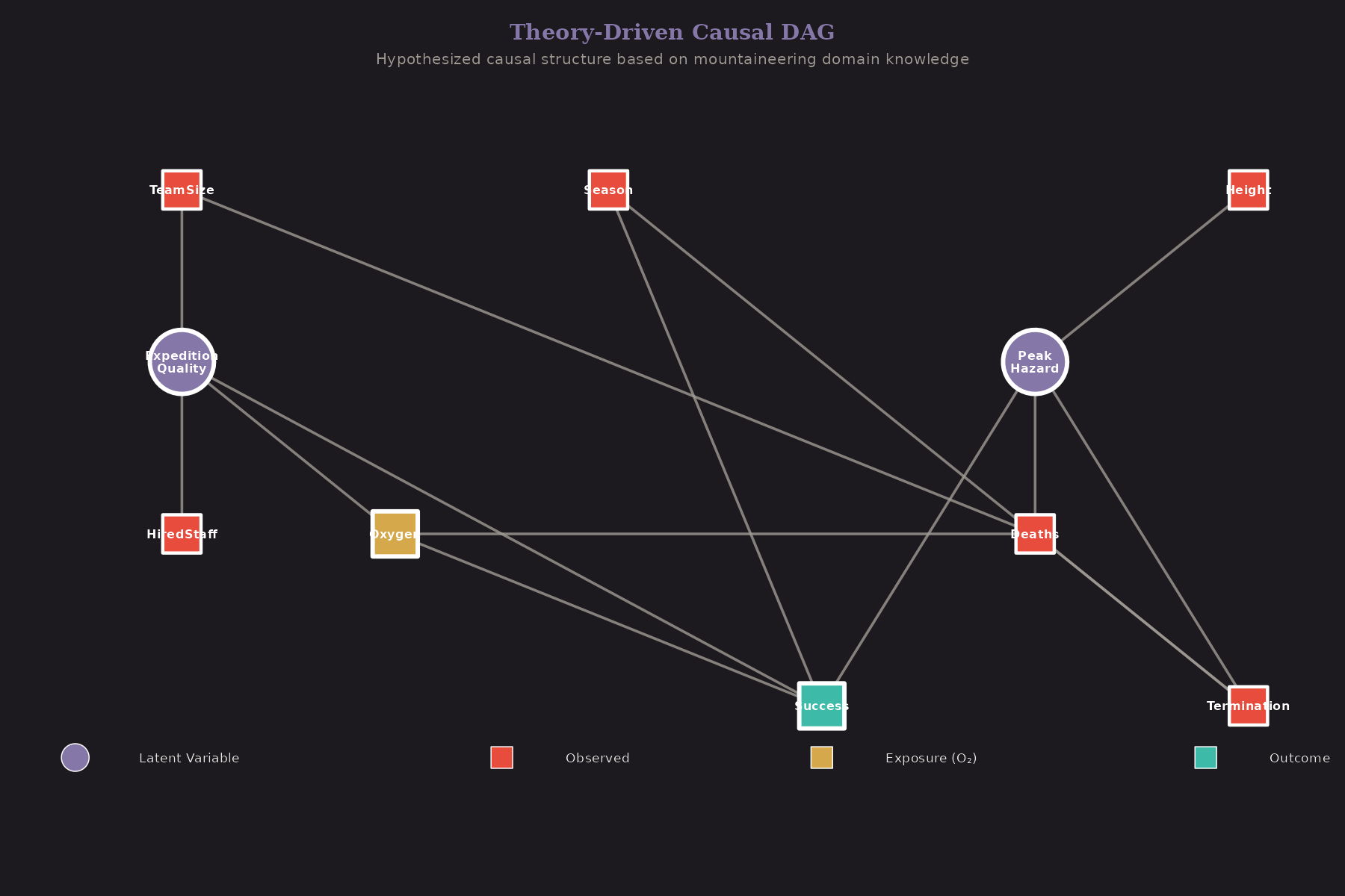
The key assumptions:
-
Expedition Quality (latent) → Oxygen Use, Team Size, Hired Staff
- Well-funded expeditions have more resources across the board
-
Peak Hazard (latent) → Success, Deaths, Termination
- Dangerous peaks affect all outcomes
-
Oxygen → Success (the effect we care about)
-
Height → Peak Hazard
- Higher peaks are more dangerous
-
Season → Success, Termination
- Weather affects outcomes
The latent variables (shaded) aren't directly observed, but we can infer them from their manifestations.
D-Separation and Adjustment Sets
The DAG tells us what we need to control for. To estimate Oxygen → Success:
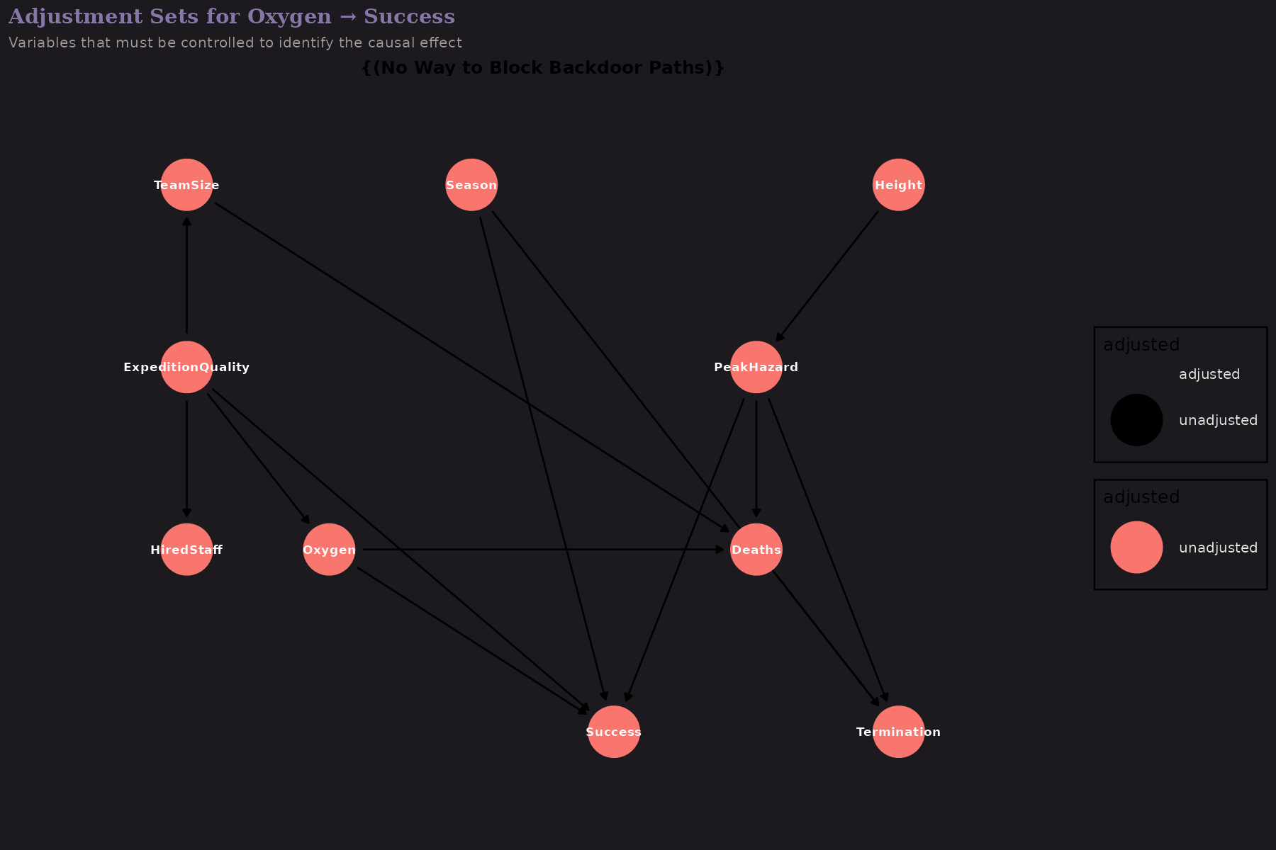
D-separation is a graphical criterion for conditional independence. If we condition on the right variables, we "block" backdoor paths that would confound our estimate.
The adjustment set for Oxygen → Success includes Expedition Quality (or its manifestations). Without controlling for quality, we'd conflate "oxygen helps" with "well-funded expeditions succeed."
Paths from Oxygen to Success
All paths connecting treatment to outcome:
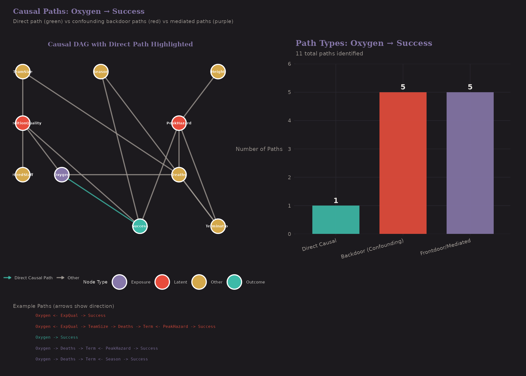
- Direct path: Oxygen → Success (the causal effect)
- Backdoor paths: Through Expedition Quality
To identify the causal effect, we need to block all backdoor paths while leaving the direct path open.
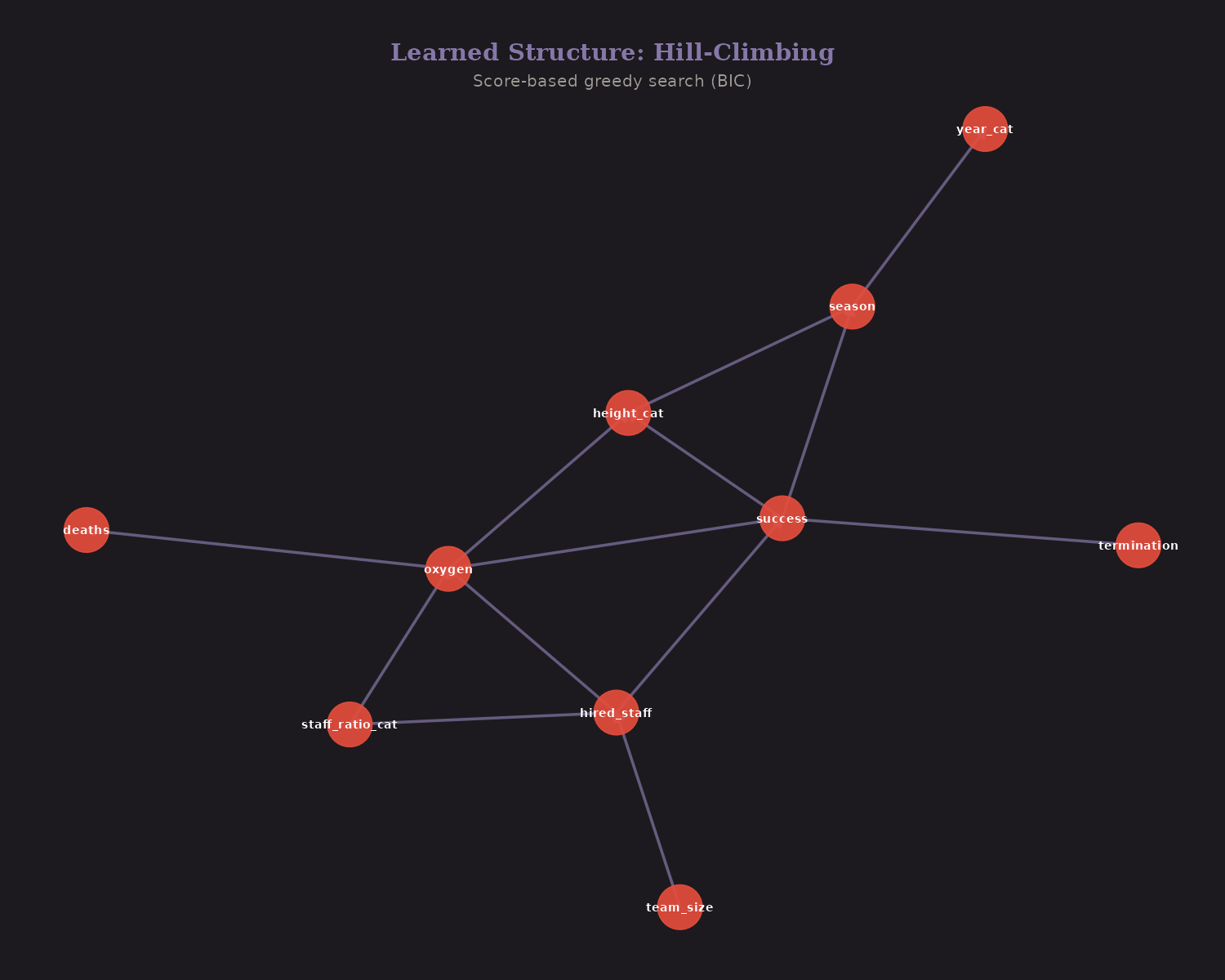
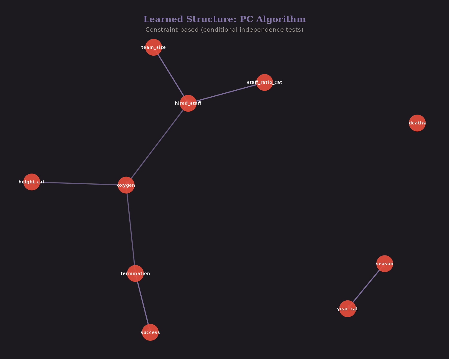
Bayesian Network Structure Learning
What if we don't know the structure? We can learn it from data.
Three algorithms:
| Algorithm | Type | Edges Found |
|---|---|---|
| Hill-Climbing | Score-based (BIC) | 13 |
| PC | Constraint-based | 7 |
| MMHC | Hybrid | 7 |
Hill-Climbing (score-based): Greedily adds/removes edges to maximize BIC score.
PC Algorithm (constraint-based): Uses conditional independence tests to discover edges.
MMHC (hybrid): Combines constraint-based skeleton discovery with score-based orientation.
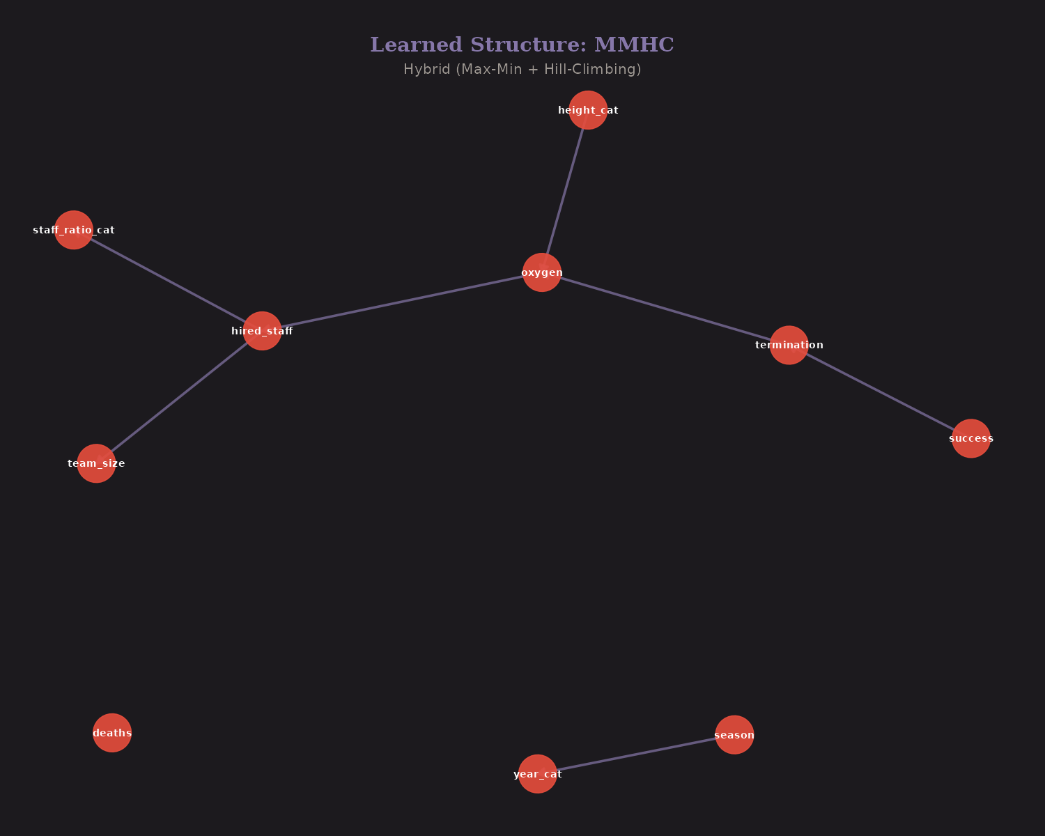
Important caveat: structure learning recovers dependencies, not causal direction. Edge orientations can flip without strong domain constraints, and discretization can induce artifacts. Treat learned graphs as hypotheses, not causal conclusions.
Edges found by ≥2 methods are robust: hired_staff → staff_ratio, season → year, success → termination, hired_staff → oxygen, oxygen → height_cat, team_size → hired_staff.
Bootstrap Edge Strength
How confident are we in each learned edge?
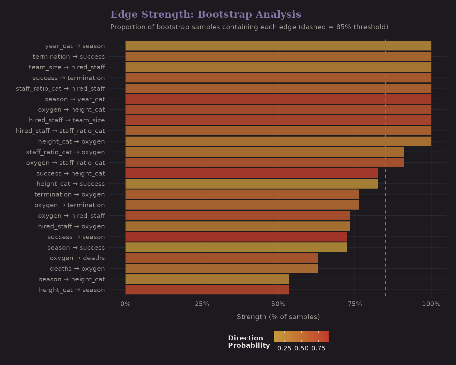
Bootstrap analysis resamples the data 200 times and checks which edges appear consistently. Edges above the 85% threshold (dashed line) are well-supported.
Strong edges include:
- Height → Success
- Oxygen → Success
- Team composition → Outcomes
These match our theory-driven expectations—reassuring.
Marginal Probabilities
The fitted Bayesian network gives us conditional probability tables. Here are the marginal probabilities:
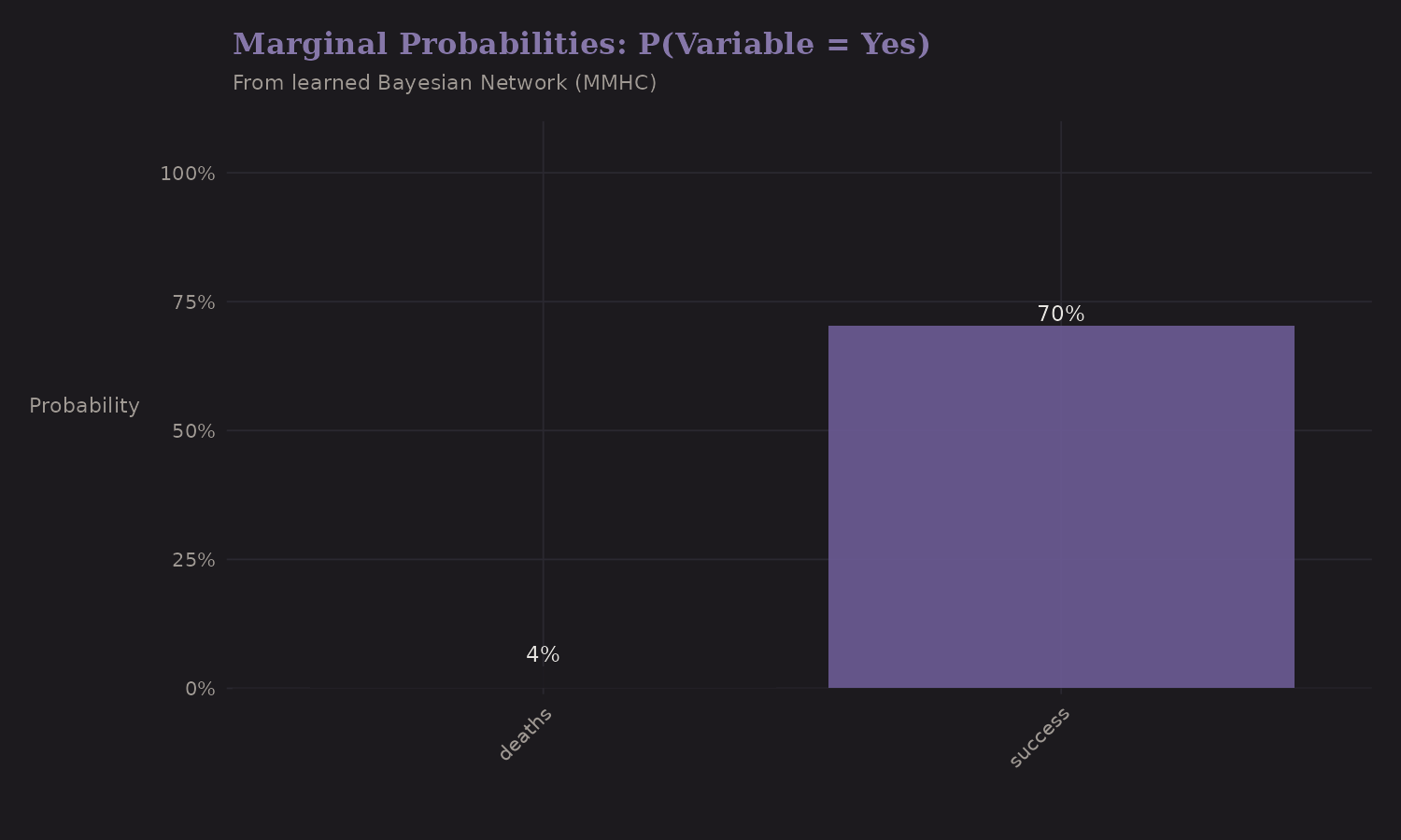
These are unconditional rates: what fraction of expeditions use oxygen, succeed, experience deaths, etc. The network structure tells us how these relate to each other conditionally.
Structural Equation Model (Exploratory)
SEMs go beyond Bayesian networks by explicitly modeling latent variables.
Note: As we'll see below, this SEM shows poor fit. The results are exploratory and shouldn't be used for causal conclusions.
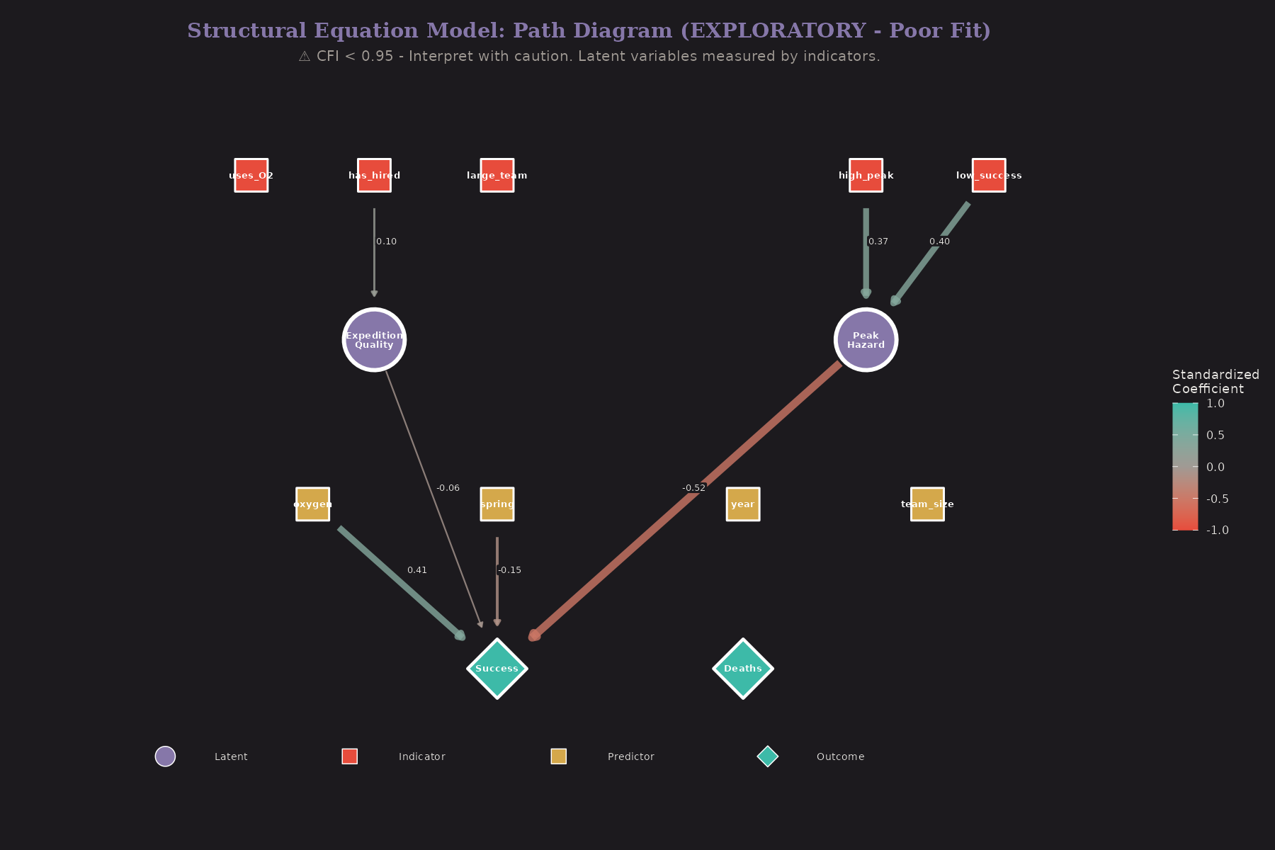
Two latent constructs:
Expedition Quality manifests through:
- Uses oxygen (indicator)
- Has hired staff (indicator)
- Large team (indicator)
Peak Hazard manifests through:
- High peak (indicator)
- Low success peak (indicator)
The structural model relates these latent variables to outcomes. This separates measurement (how we observe the latent) from structure (how latents relate to each other).
Factor Loadings
How strongly do indicators reflect the latent constructs?
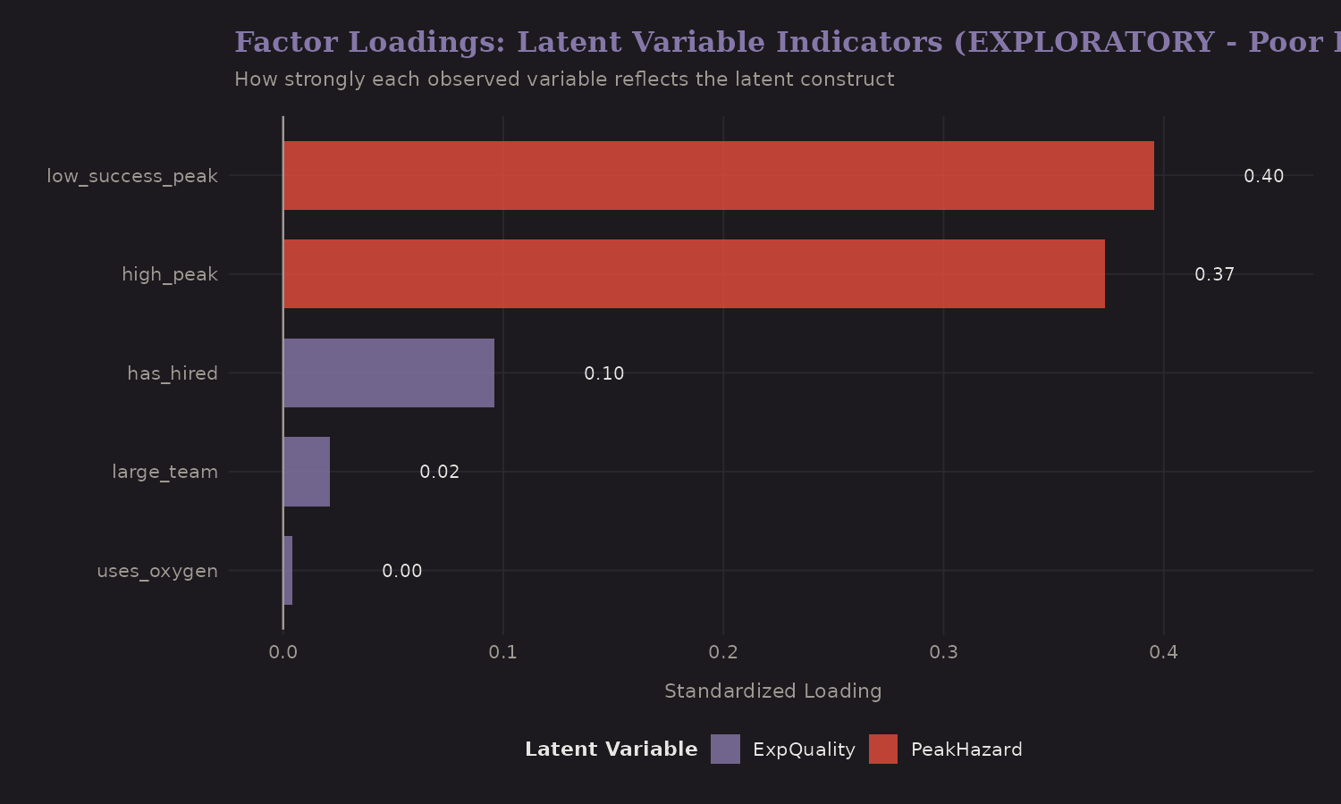
Higher loadings mean stronger indicators. For Expedition Quality, oxygen use and hired staff load strongly—they're good proxies for overall preparation.
SEM Effects on Success
What predicts summit success in the structural model?
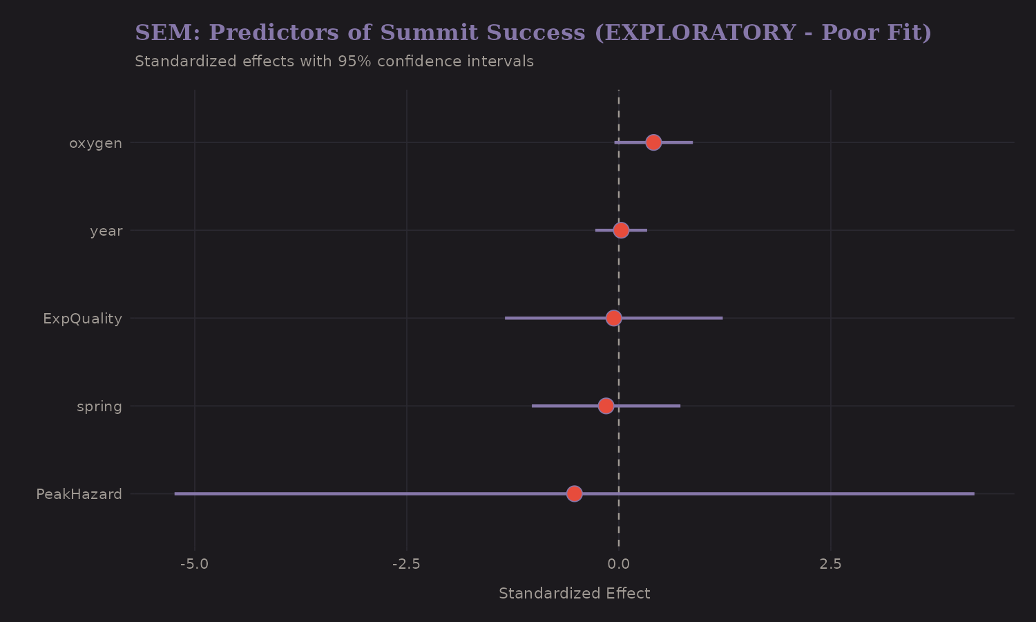
The standardized effects:
| Predictor | Effect on Success |
|---|---|
| Peak Hazard | -0.52 |
| Oxygen | +0.41 |
| Spring season | -0.15 |
| Expedition Quality | -0.06 |
Peak Hazard has the strongest (negative) effect. Oxygen has a direct positive effect (+0.41) even after accounting for the latent quality construct. This decomposition is useful: oxygen works partly through quality (better expeditions use it) and partly directly (physiologically).
Model Fit
Does the SEM fit the data well?
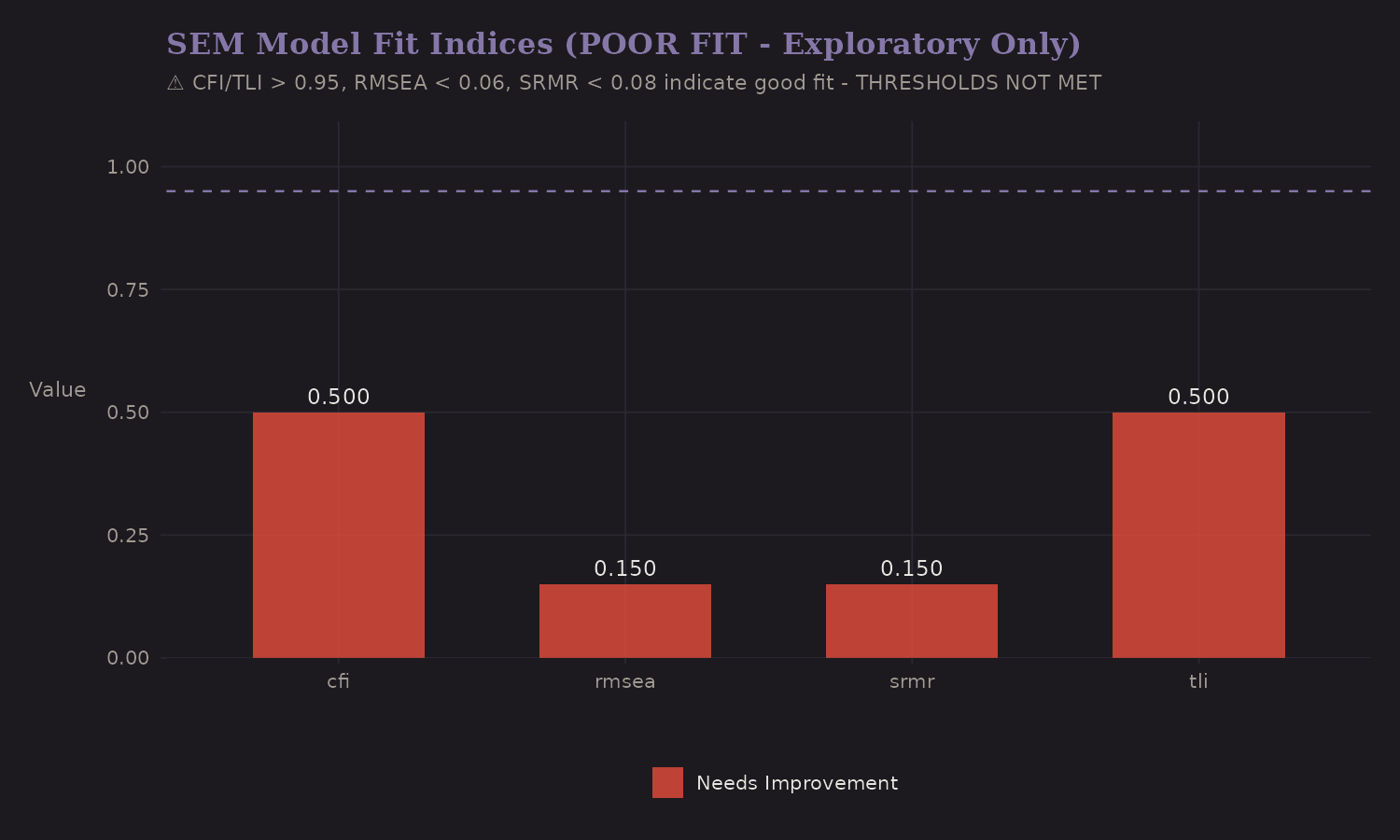
Standard fit indices:
| Measure | Value | Threshold | Status |
|---|---|---|---|
| CFI | 0.50 | > 0.95 | Poor |
| RMSEA | 0.15 | < 0.06 | Poor |
The model fit is poor by conventional standards. This is a limitation: our stylized two-factor latent structure doesn't fully capture the complexity of real expedition data. The SEM provides useful conceptual decomposition, but shouldn't be trusted for precise effect estimates.
Probabilistic Inference
With a fitted network, we can answer "what if" questions:
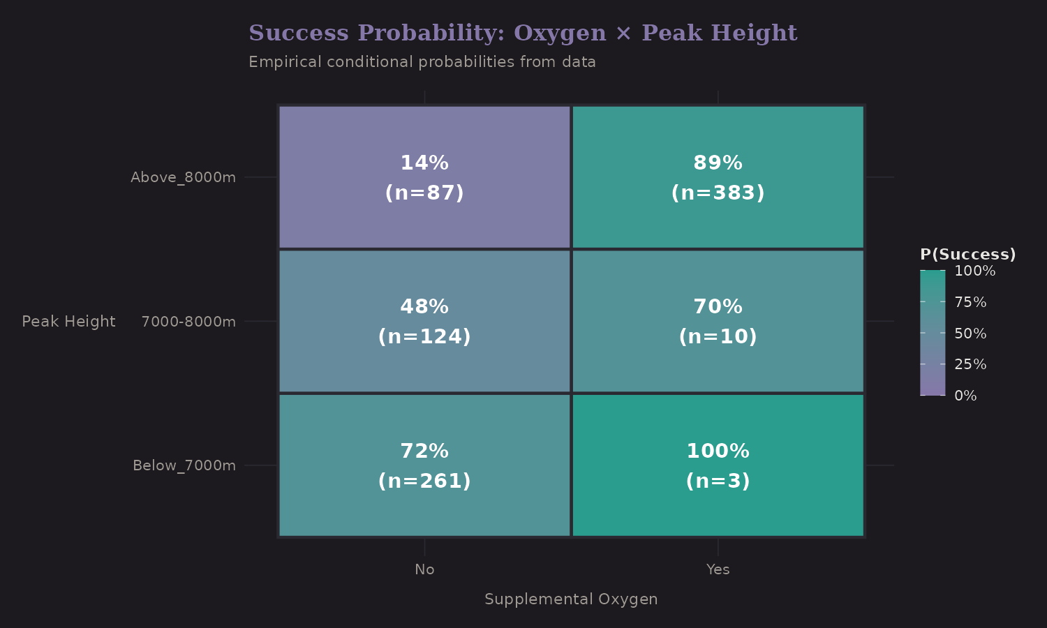
This grid shows P(Success | Oxygen, Height Category). Key conditional probabilities from the fitted network:
| Scenario | P(Success) |
|---|---|
| O2 = Yes, Height = 8000m+ | 89% |
| O2 = No, Height = 8000m+ | 14% |
| Oxygen effect at 8000m+ | +76 pp |
The oxygen benefit is largest on 8000m+ peaks—a 76 percentage point difference. This is consistent with physiology: severe hypoxia at extreme altitude makes supplemental oxygen critical.
Risk Profiles
Different expedition types have different risk/reward profiles:
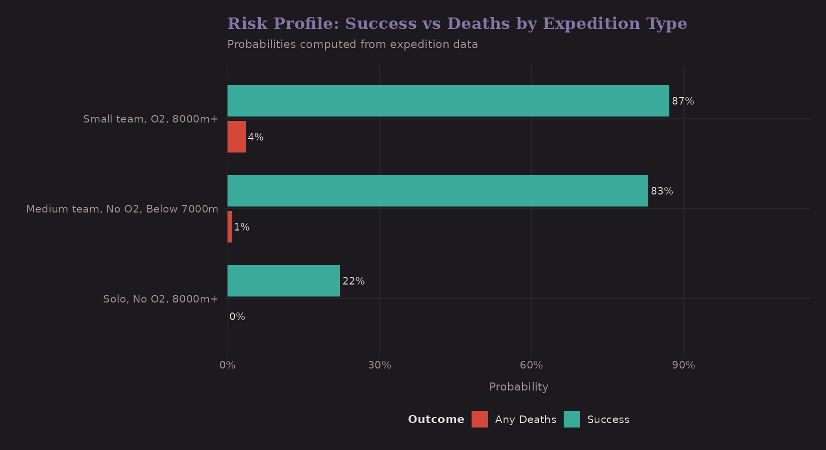
Sample risk profiles from the network:
| Expedition Type | P(Success) | P(Deaths) |
|---|---|---|
| Solo, No O2, 8000m+ | 22% | ~0% |
| Small team, O2, 8000m+ | 87% | 4% |
Large teams with oxygen on mid-altitude peaks have high success and low death rates. Solo attempts without oxygen on 8000m+ peaks are... risky. (Death rates are underestimated due to rare event sparsity.)
Structure Comparison
Do theory-driven and data-learned structures agree?
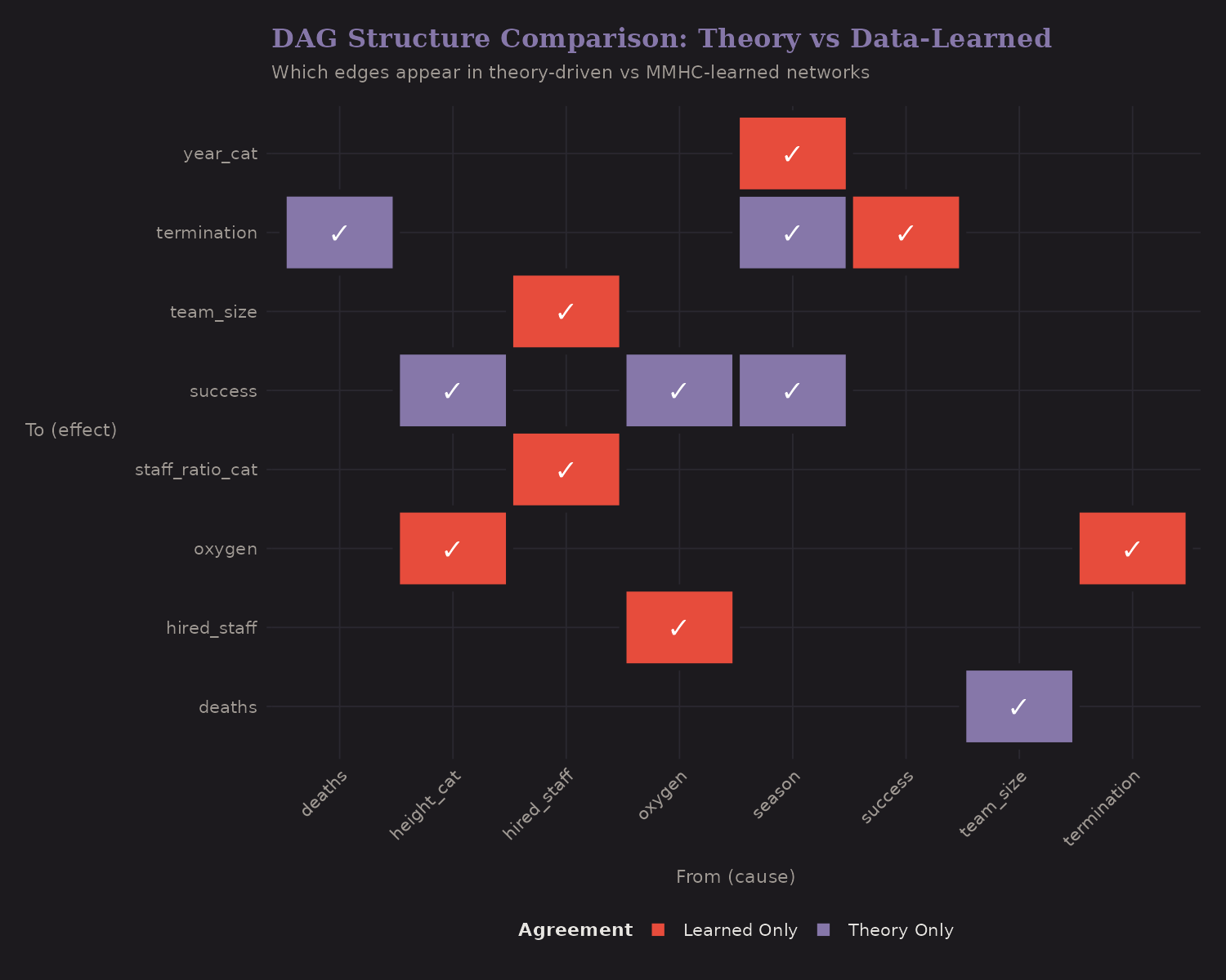
- Both (green): Edges found in theory AND learned from data
- Theory Only (purple): We expected but data didn't strongly support
- Learned Only (red): Data found but we didn't theorize
Agreement is reassuring. Disagreements suggest either theory needs updating or data has quirks.
Latent Variable Distributions
The SEM estimates factor scores for each expedition:
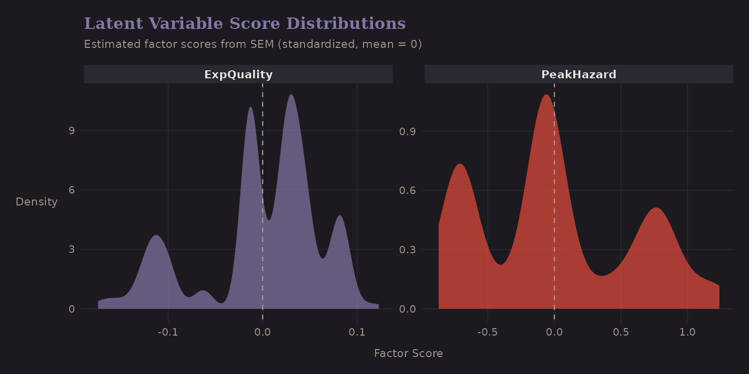
Expedition Quality and Peak Hazard are approximately normally distributed (by design—SEMs assume this). The zero point is the mean; positive scores indicate above-average quality or hazard.
Latent Space and Outcomes
Plotting expeditions in latent space reveals structure:
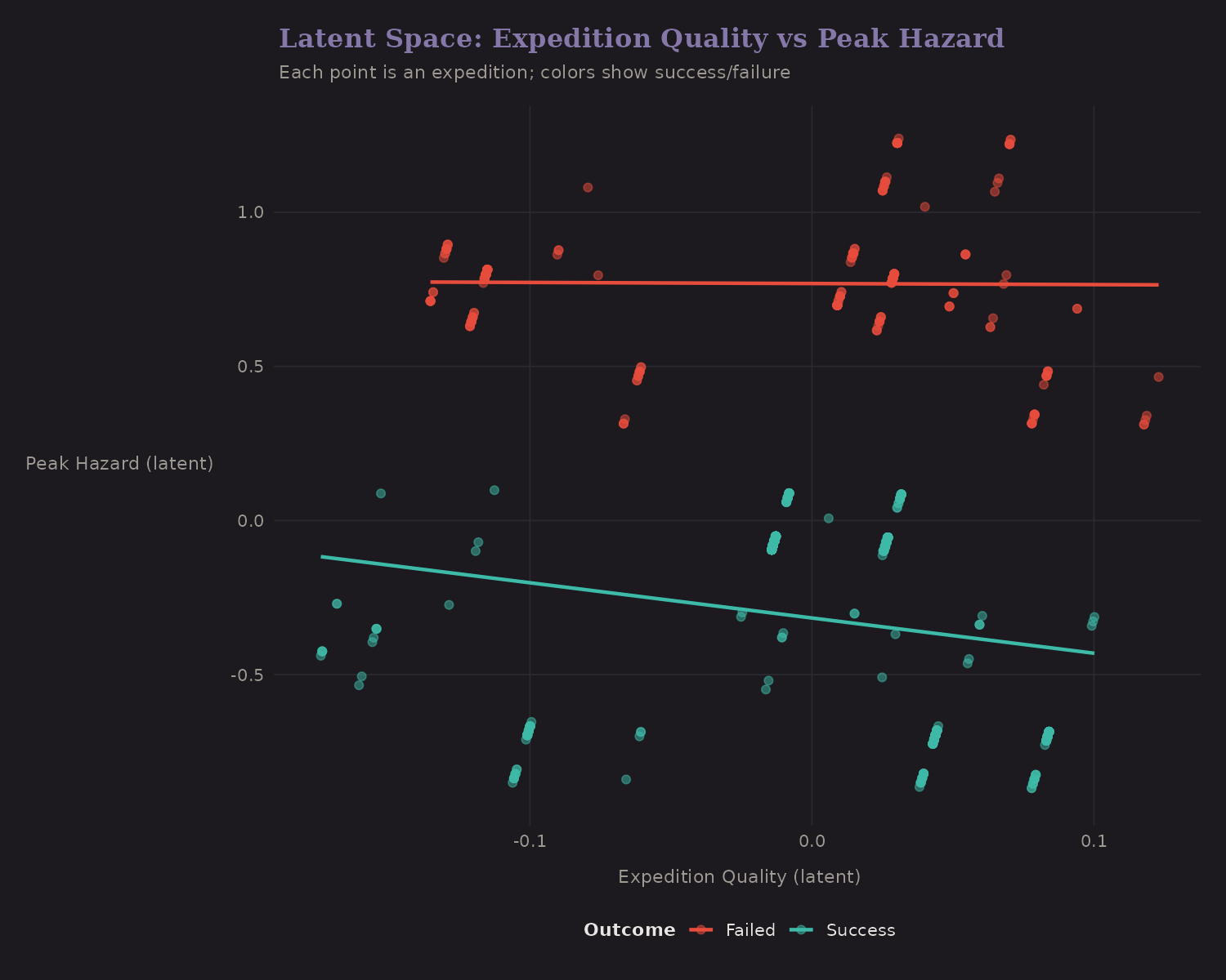
- High Quality + Low Hazard: High success (blue cluster, upper left)
- Low Quality + High Hazard: Low success (orange, lower right)
The linear fits show that both latent dimensions predict success, but Expedition Quality has a stronger separation.
What I Learned
A few takeaways from PGM analysis:
-
Making assumptions explicit helps. Drawing the DAG forces you to articulate what you believe about causal structure.
-
Structure learning validates theory. When data-learned edges match theory, we have convergent evidence.
-
Latent variables capture unobservables. "Expedition Quality" isn't directly measured, but we can infer it from indicators.
-
Adjustment sets matter. The DAG tells us what to control for. Without it, we might under- or over-adjust.
-
PGMs aren't causal inference. They encode assumptions and compute conditional probabilities. Estimating causal effects requires additional methods—covered in the next post.
Limitations
A few important caveats:
-
DAG encodes assumptions, doesn't prove them. The DAG reflects my beliefs about causal structure. Data can support or refute edges, but can't prove causation.
-
Structure learning finds associations, not necessarily causes. A learned edge A → B might be B → A or A ← C → B in reality.
-
SEM fit was poor (CFI = 0.50). The latent variable results are exploratory. The two-factor structure may be too simplistic.
-
Bayesian Network is more reliable here. For structural insights, trust the BN over the SEM.
Resources
If you want to go deeper:
- Pearl: Causality and The Book of Why—foundational texts on causal DAGs
- Koller & Friedman: Probabilistic Graphical Models—comprehensive treatment
- dagitty: R package for DAG specification and analysis
- bnlearn: R package for Bayesian network structure learning
- lavaan: R package for structural equation modeling
The next post applies these ideas to estimate causal effects using propensity scores, doubly robust estimation, and causal forests.