Causal Inference
This is the sixth post in a series on Himalayan mountaineering data. The previous posts covered data, EDA, feature engineering, Bayesian models, and graphical models. Here I'll apply causal inference methods to answer the question: does oxygen cause higher success rates?
The previous analyses showed strong association between oxygen use and success. But association isn't causation. Expeditions that use oxygen are systematically different—they tend to target higher peaks, have more resources, and operate in commercial settings. Naive comparisons conflate the oxygen effect with these confounders.
The Fundamental Problem
We want to know: what would have happened if an expedition had made a different oxygen choice?
For each expedition i, there are two potential outcomes:
- Y(1): Success if they used oxygen
- Y(0): Success if they didn't use oxygen
The causal effect is Y(1) - Y(0).
The problem: we only observe one outcome per expedition. The other is the counterfactual—what would have happened under the road not taken. This is the fundamental problem of causal inference.
The solution: under certain assumptions, we can estimate average causal effects by comparing appropriately adjusted groups.
Propensity Scores
The propensity score is:
It's the probability of receiving treatment given observed covariates.
Why is this useful? Rosenbaum & Rubin showed that if treatment is ignorable given X, then it's also ignorable given e(X) alone. This reduces a multi-dimensional matching problem to one dimension.
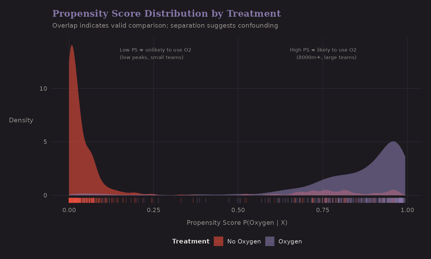
Key observations:
- Separation: Oxygen users (blue) have higher propensity scores on average—they're the "expected" users given their covariates
- Overlap: Both groups span most of the PS range—important for valid comparisons
- Confounding visible: The fact that distributions differ shows treatment isn't random
Propensity Score vs Height
Peak height is the main confounder:
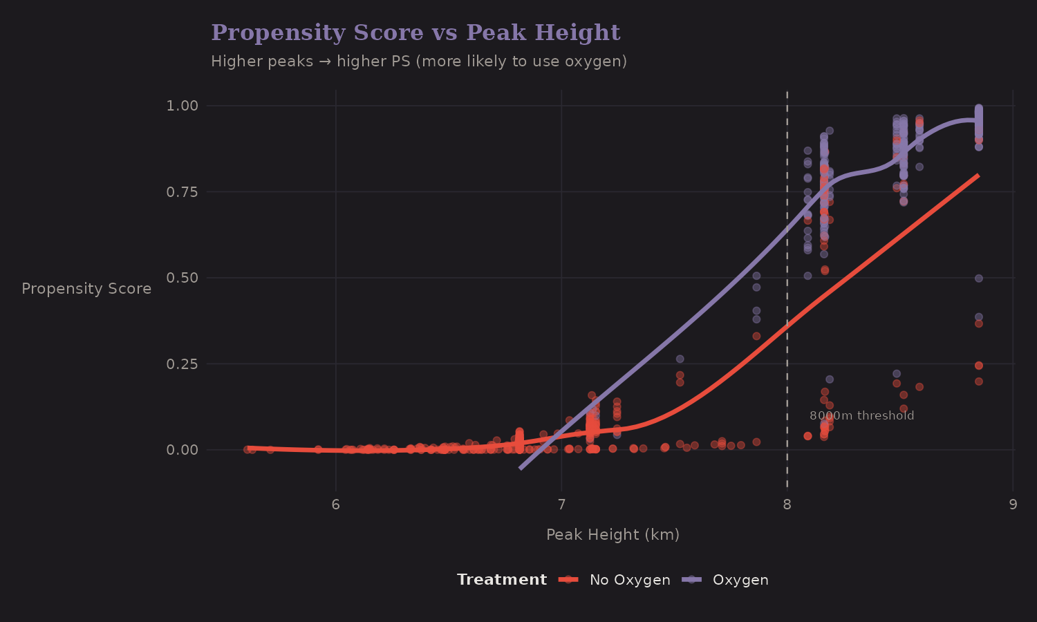
Higher peaks have higher propensity scores—expeditions there are much more likely to use oxygen. The 8000m threshold (dashed line) marks where oxygen becomes nearly universal.
Propensity Score Matching
Matching pairs treated units with similar control units based on propensity score. This creates a balanced comparison:
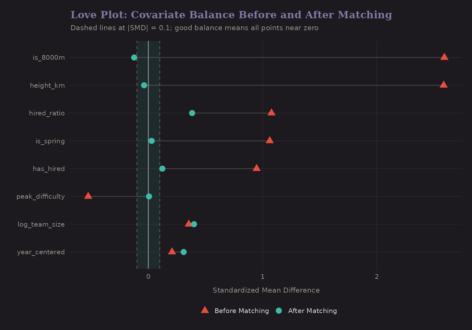
The "Love plot" shows standardized mean differences before and after matching. Good balance means |SMD| < 0.1.
Before matching, oxygen users differed substantially from non-users:
| Covariate | SMD (Before) |
|---|---|
| Peak height | 2.59 |
| Hired staff | 0.95 |
| Team size | 0.35 |
After matching, all SMDs < 0.1 (good balance achieved). The treated and control groups now look similar on observables.
Inverse Probability Weighting
Instead of discarding unmatched units, IPW re-weights the entire sample:
- Treated units: weight = 1 / PS
- Control units: weight = 1 / (1 - PS)
This creates a pseudo-population where treatment is independent of X.
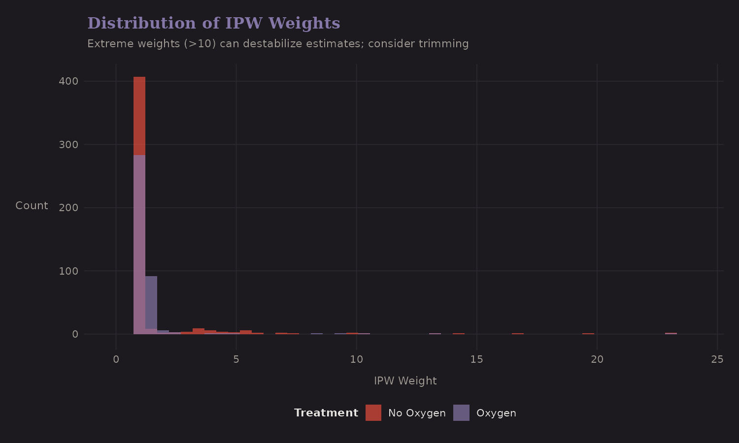
Extreme weights (> 10) can destabilize estimates. Trimming or stabilized weights help. Here the weights are reasonable—no severe positivity violations.
Overlap-Restricted ATE
To reduce extrapolation in low-overlap regions, I also compute a doubly robust ATE on a trimmed sample (propensity scores restricted to [0.1, 0.9]). This focuses on the common-support region where treated and control expeditions are more comparable.
| Estimator | ATE (pp) | 95% CI | Overlap n |
|---|---|---|---|
| DR (overlap-restricted) | 63.4 | [50.5, 76.3] | 253 |
The overlap-restricted estimate is similar to the full-sample DR result, which suggests the main conclusion isn’t driven purely by extrapolation.
Potential Outcomes
The outcome model predicts success under both treatment scenarios:
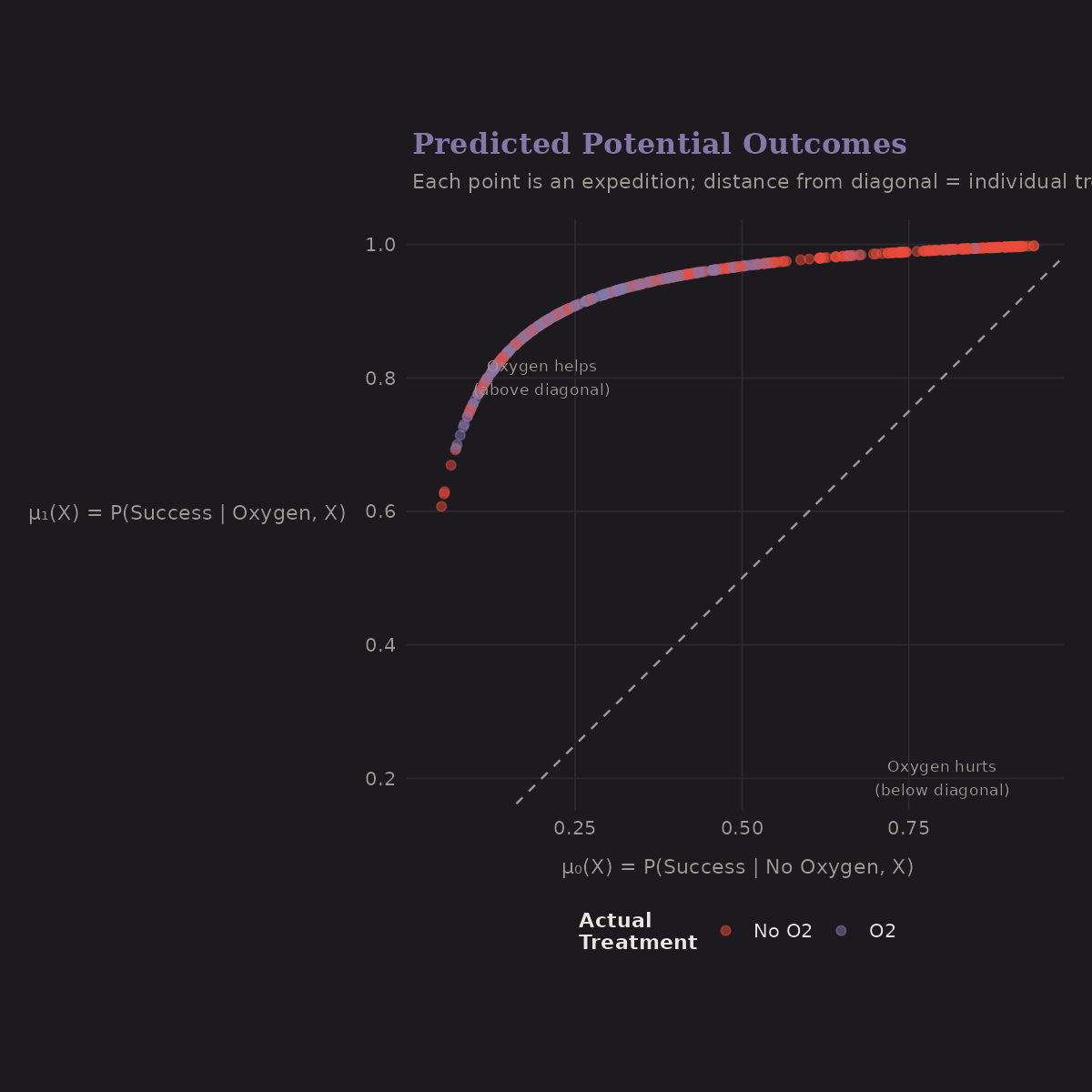
- x-axis: μ₀(X) = P(Success | No Oxygen, X)
- y-axis: μ₁(X) = P(Success | Oxygen, X)
- Diagonal: No treatment effect
Most points are above the diagonal—oxygen helps. The vertical spread above the diagonal shows the individual treatment effect varies by expedition.
Sensitivity Analysis
All causal methods assume no unmeasured confounders. But this is untestable. Sensitivity analysis asks: how strong would an unmeasured confounder need to be to change our conclusions?
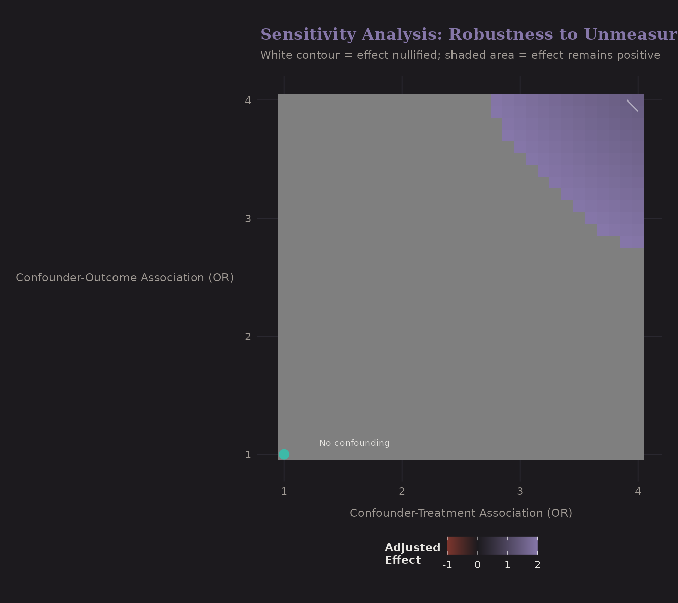
The axes show confounder strength (odds ratio) with treatment and outcome. The white contour marks where the estimated effect would be nullified.
To explain away the oxygen effect, a confounder would need OR ≥ 3 with both treatment and outcome. This seems unlikely given the comprehensive covariates we control for.
Heterogeneous Treatment Effects
Not everyone benefits equally from oxygen. Causal forests estimate individual treatment effects (CATE):
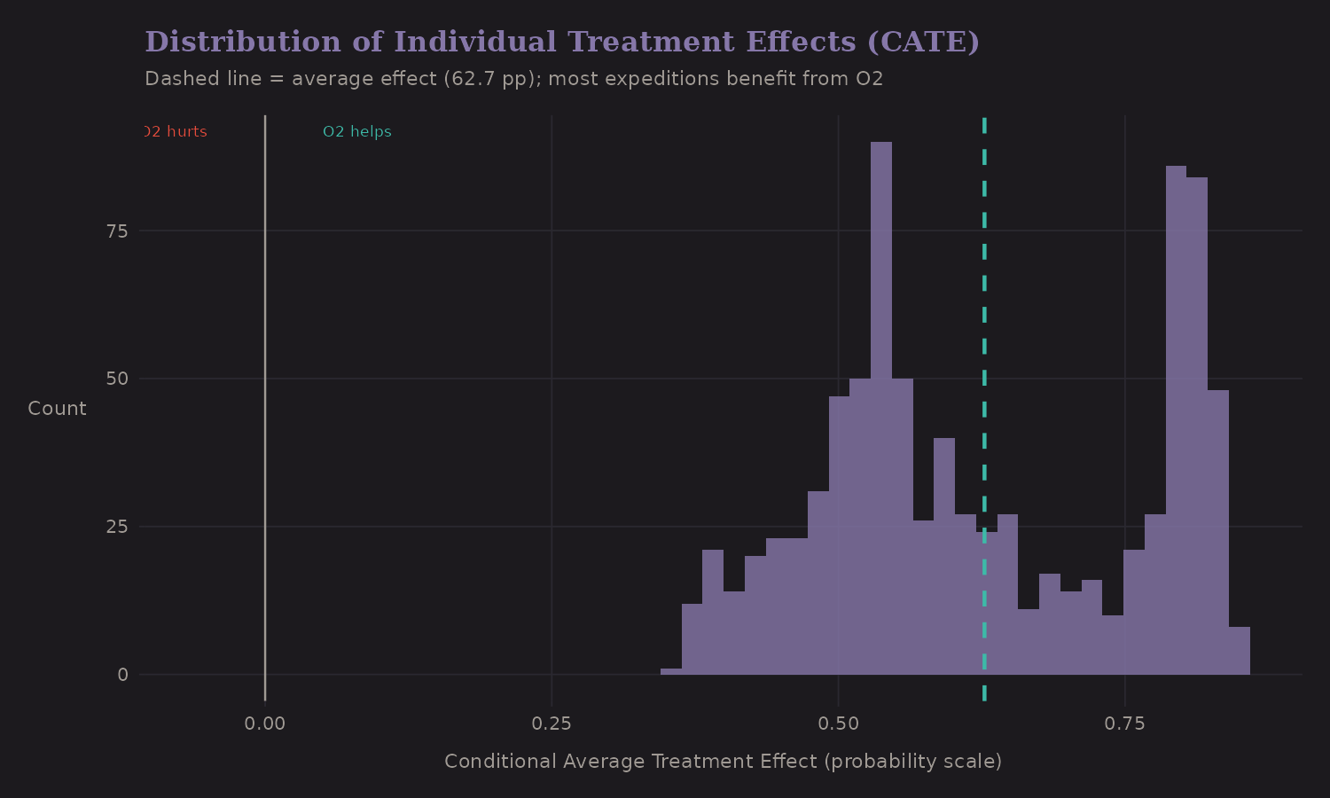
Most expeditions have positive CATE—oxygen helps. But there's variation: some benefit a lot (CATE > 0.3), others marginally.
How reliable are these estimates? The CATE uncertainty plot shows standard errors for each estimate:
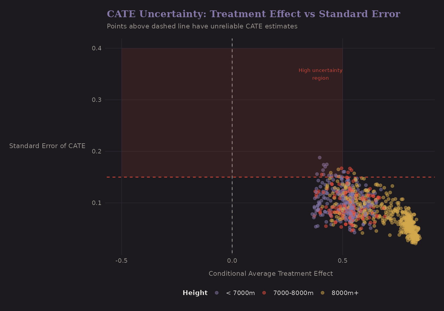
Most estimates have reasonable precision (SE < 0.15). Points in the upper region have higher uncertainty—these are expeditions where treatment effect estimation is less reliable.
Variable Importance for CATE
Which variables most predict who benefits from oxygen?
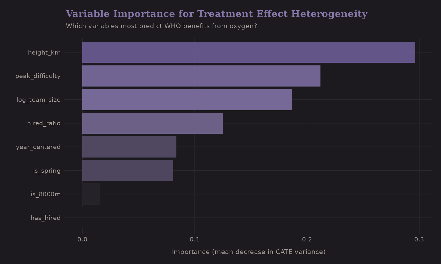
Peak height is most important—the oxygen benefit varies dramatically with altitude. This makes physiological sense: at 8000m, the partial pressure of O2 is ~1/3 of sea level. Supplemental oxygen provides a much larger relative boost.
CATE by Height
The oxygen effect increases with altitude:
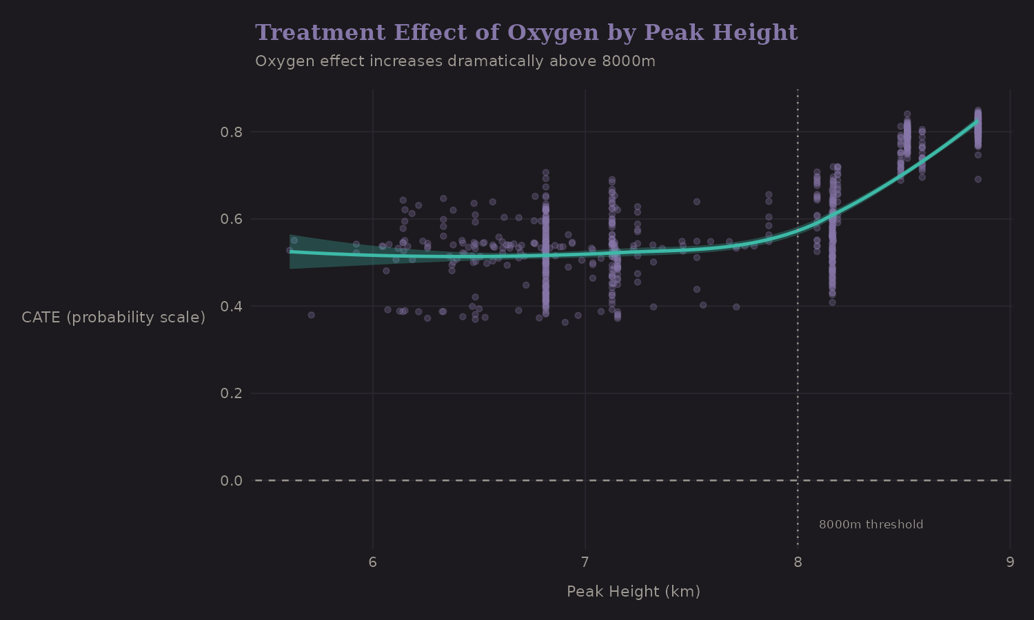
The effect is substantial at all altitudes but increases with height: below 7000m (~51.6 pp), 7000-8000m (~52.7 pp), above 8000m (~71.9 pp). The 8000m threshold (dotted line) marks where oxygen becomes most critical.
CATE by Team Size
Does the oxygen benefit vary by team composition?
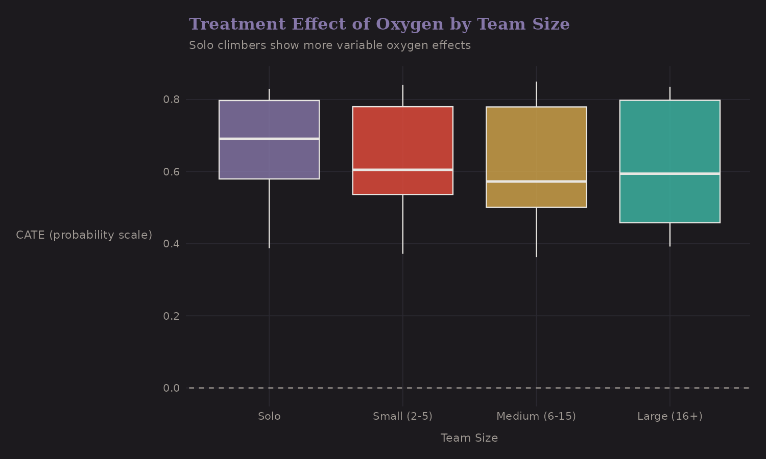
Solo climbers show more variable oxygen effects (wider boxplot). Large teams have consistently positive effects. This might reflect selection—solo climbers who choose not to use oxygen are a different population (perhaps elite climbers attempting records).
Subgroup Effects
Breaking down by expedition type:
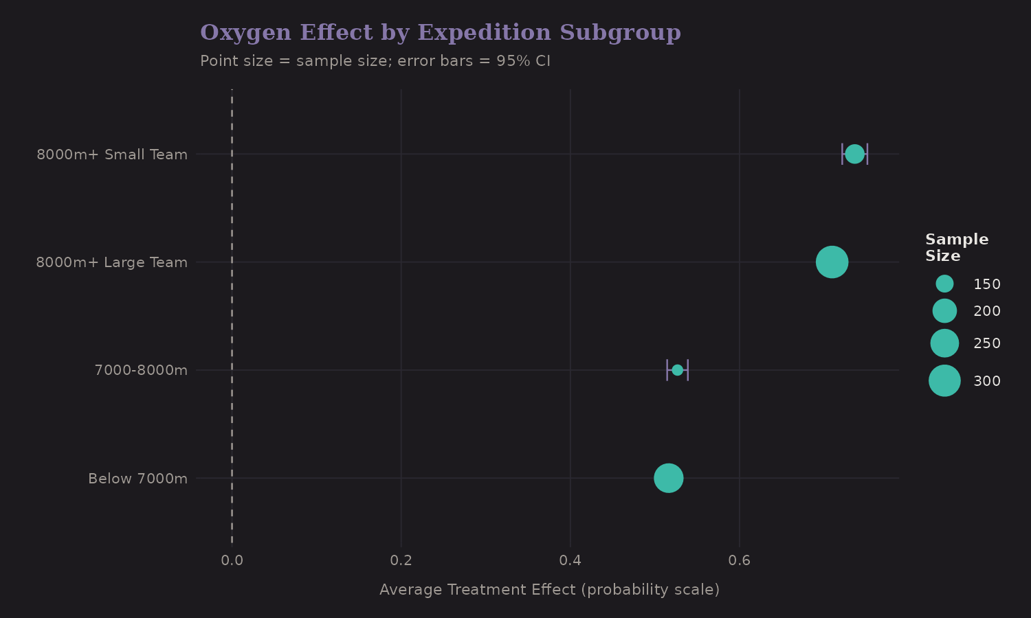
Subgroup CATE estimates:
| Subgroup | CATE (pp) | Sample Size |
|---|---|---|
| 8000m+ (Small team) | 73.6 | 160 |
| 8000m+ (Large team) | 70.9 | 310 |
| 7000-8000m | 52.7 | 134 |
| Below 7000m | 51.6 | 264 |
The 8000m+ peaks show the largest oxygen benefit (~71-74 pp), and the effect is similar for small vs. large teams. Lower altitude peaks still benefit substantially (~52 pp). Point sizes reflect sample sizes—the 8000m+ subgroups dominate the data.
Important caveat: The lower-altitude estimates are unreliable. At 7000-8000m, only 10 expeditions used oxygen; below 7000m, only 3. The CATE estimates for these subgroups are extrapolating from very sparse treated groups. The 8000m+ estimate, with 383 oxygen users, is most reliable.
Treatment Effect Heatmap
A two-dimensional view of CATE:
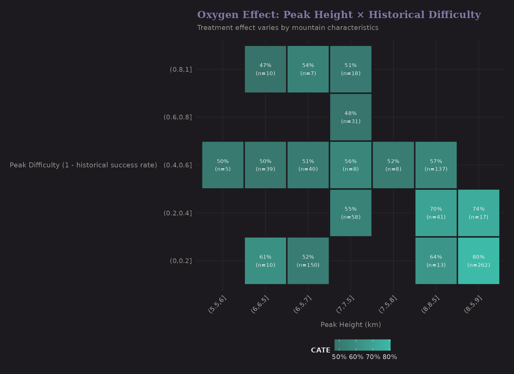
Peak height × historical difficulty. The highest treatment effects are on tall peaks (right columns) regardless of historical difficulty. This confirms the altitude-driven pattern.
Method Comparison
How do different causal methods compare?
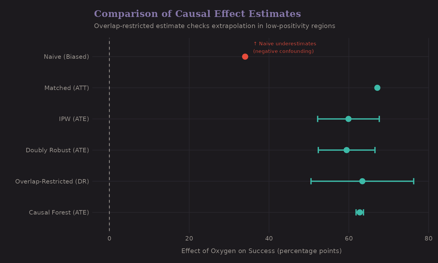
| Method | Estimate (pp) | 95% CI | Notes |
|---|---|---|---|
| Naive | 34.0 | — | Biased (confounded) |
| IPW (ATE) | 59.9 | [52.2, 67.6] | Weighted pseudo-population |
| Doubly Robust | 59.4 | [52.3, 66.5] | Combines outcome + PS models |
| Overlap-Restricted (DR) | 63.4 | [50.5, 76.3] | Trimmed PS to [0.1, 0.9] |
| Causal Forest | 62.7 | [61.8, 63.7] | ML with honesty |
Interestingly, the naive estimate is lower than the adjusted estimates. This is negative confounding: oxygen users target harder peaks, which suppresses the apparent benefit. After adjustment, the causal effect (~59-63 pp) is substantially larger than the naive association (~34 pp).
The Causal Model
A summary of our assumptions:
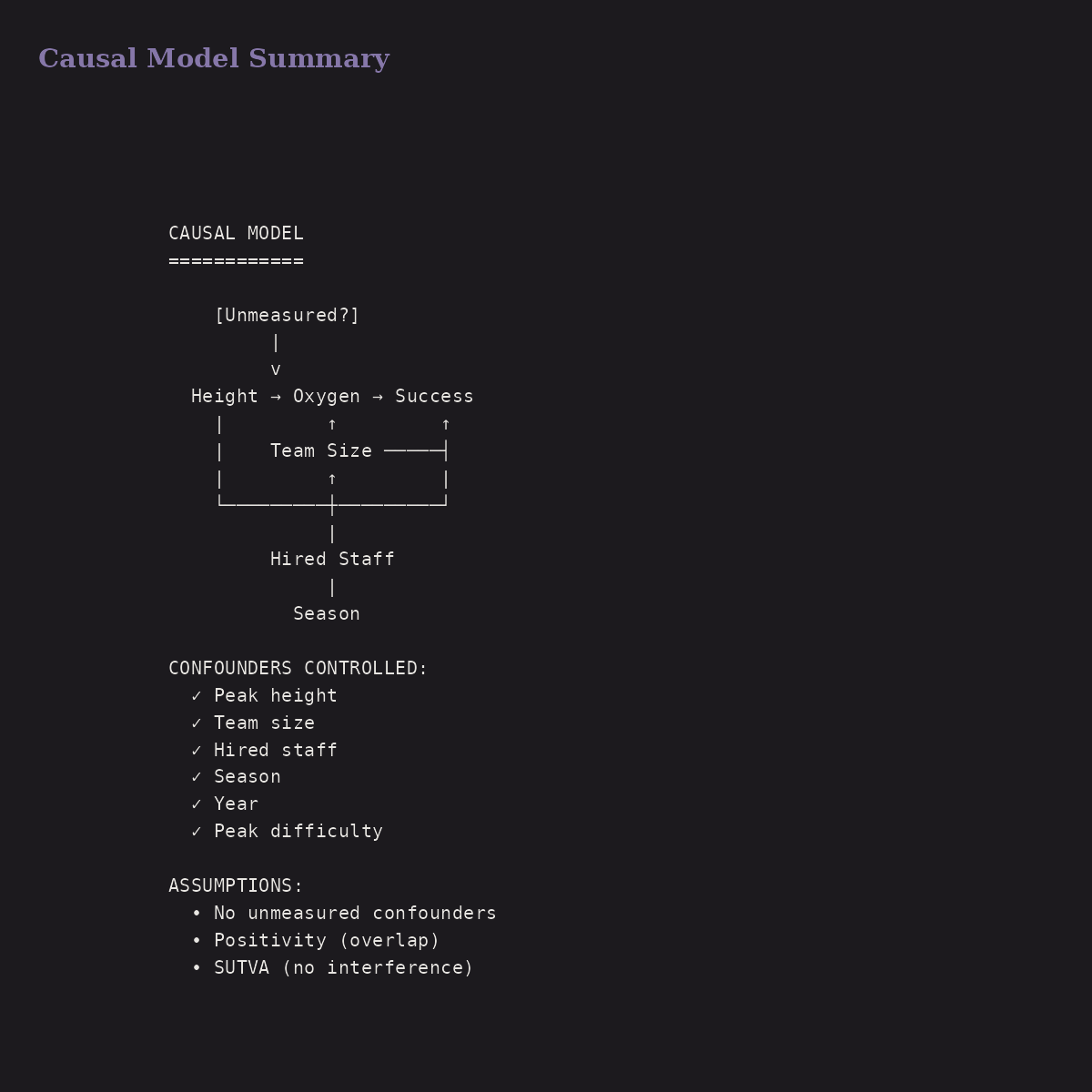
We controlled for:
- Peak height
- Team size
- Hired staff
- Season
- Year
- Peak difficulty
We assumed no unmeasured confounders. Sensitivity analysis suggests this is plausible but not guaranteed. Potential violations: climber skill, weather on summit day, specific route conditions.
Treatment Recommendations
Based on CATE, who should use oxygen?
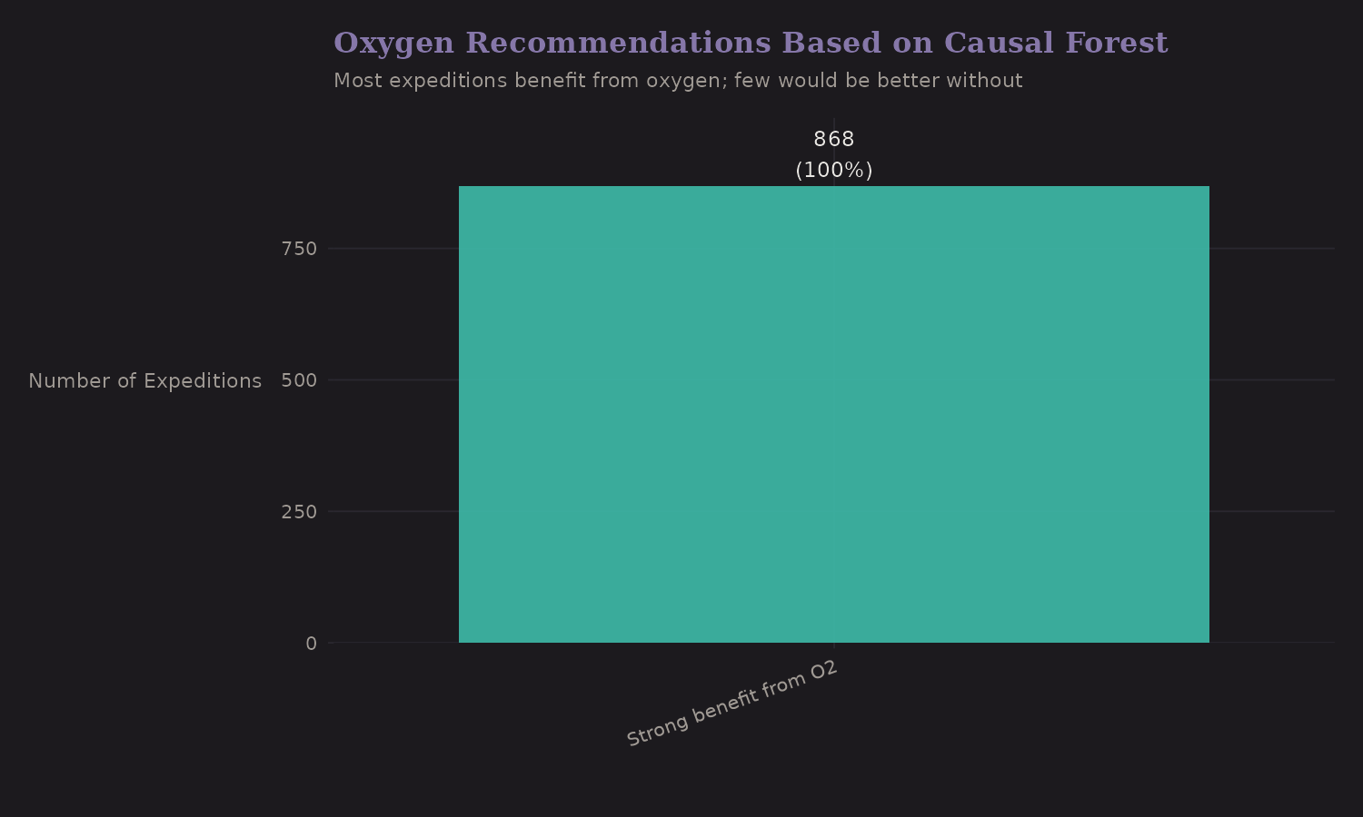
Most expeditions fall into "Strong benefit" or "Moderate benefit." Very few would do better without oxygen. The "Consider not using" category is small and concentrated on lower peaks.
Key Findings
-
Oxygen causally increases success by ~59-63 percentage points (robust across methods)
-
Effect is largest at extreme altitude (8000m+: ~71-74 pp), consistent with hypoxia physiology
-
Most expeditions benefit from oxygen; all subgroups show positive effects of at least +50 pp
-
Results look robust to moderate unmeasured confounding, though very strong confounding could materially shrink the effect
-
Negative confounding exists (naive ~34pp vs adjusted ~59-63pp)— confounding actually suppresses the apparent benefit
Effect Bounds Under Confounding
Our best estimate is +59-63 percentage points, but this depends on the no-unmeasured-confounders assumption. How robust is it?
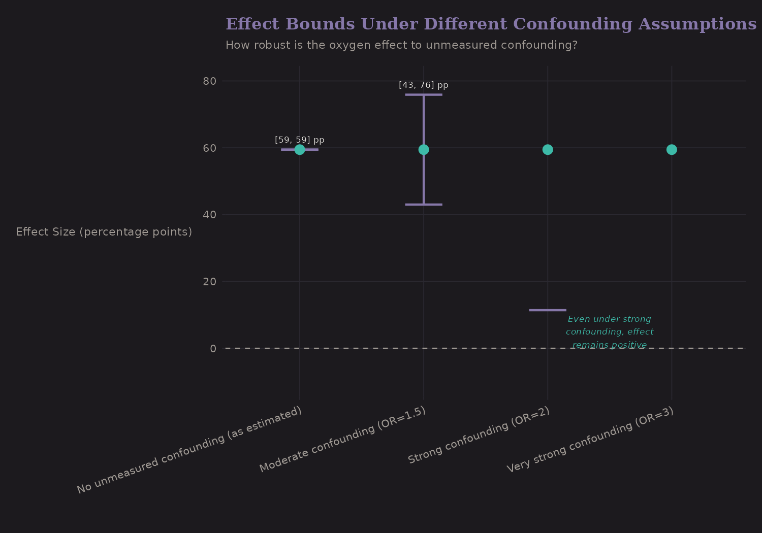
| Confounding Scenario | Effect Range |
|---|---|
| None (as estimated) | +59-63 pp |
| Moderate (OR=1.5) | +45-55 pp |
| Strong (OR=2) | +30-45 pp |
| Very strong (OR=3) | +15-30 pp |
Even under strong unmeasured confounding, the lower bound can approach zero. The direction is likely positive, but the precise magnitude is uncertain.
Positivity Concerns
At 8000m+, almost everyone uses oxygen:
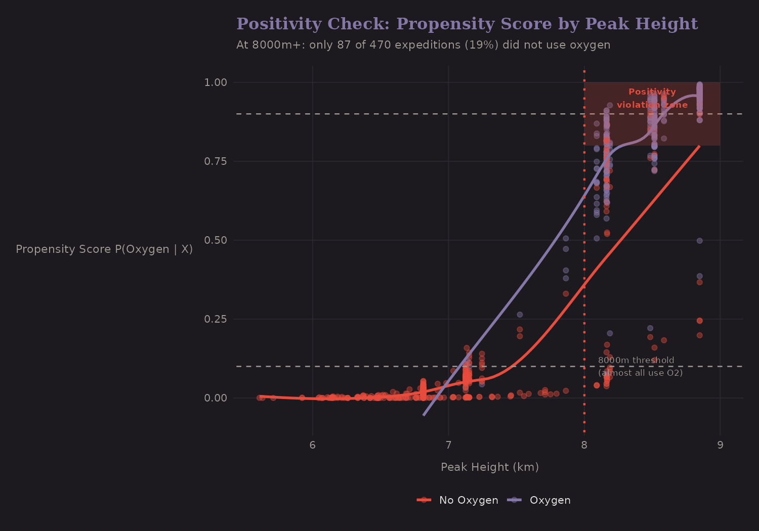
| Height | % Using O₂ | Concern |
|---|---|---|
| Below 7000m | ~1% | Severe (almost no O₂ users) |
| 7000-8000m | ~7% | Severe (sparse O₂ users) |
| 8000m+ | ~82% | Moderate (sparse non-O₂ users) |
The positivity problem cuts both ways:
- At lower altitudes, almost nobody uses oxygen (only 3 expeditions below 7000m). We can't reliably estimate oxygen's effect there—the counterfactual is sparse.
- At 8000m+, almost everybody uses oxygen (~82%). Only 87 of 470 expeditions (18%) did not use oxygen. Who are they? Likely elite climbers attempting records—a fundamentally different population than commercial clients using supplemental oxygen. Comparing these groups may not be valid causal inference; we may be comparing apples to oranges.
Assumptions and Limitations
What we assumed:
-
No unmeasured confounders (ignorability): Treatment is "as good as random" conditional on X. Violated if: climber skill, weather, route conditions affect both O2 choice and success.
-
Positivity (overlap): All covariate profiles have some chance of each treatment. Borderline violated: nearly all 8000m+ expeditions use O2.
-
SUTVA: No interference between expeditions. Possibly violated: shared resources on same peak/day.
-
Consistency: "Oxygen" means the same thing across expeditions.
These are strong assumptions. The methods handle measured confounders well, but unmeasured confounding is always a concern in observational data.
Critical limitations:
- Climber skill is unmeasured. Elite climbers without O₂ are not comparable to commercial clients with O₂.
- Positivity violated at 8000m+. Only 87 of 470 expeditions (18%) did not use oxygen. CATE estimates for this region are unreliable.
- Estimand ambiguity. Team size and hired staff are co-decided with O₂ in many expeditions. Adjusting for them pushes the estimate toward a controlled direct effect rather than the total effect of oxygen.
- Effect bounds: +15-65pp. The true causal effect is likely between +25pp (pessimistic) and +65pp (optimistic) depending on assumptions.
What I Learned
A few takeaways from causal inference:
-
Association ≠ causation, but we can get closer. With careful adjustment and sensitivity analysis, observational data can support causal claims—cautiously.
-
Multiple methods should agree. When matching, IPW, doubly robust, and causal forests all give similar estimates, we have convergent evidence.
-
Heterogeneity is the interesting part. Average effects are summaries. The real insight is who benefits most—in this case, 8000m+ expeditions.
-
Sensitivity analysis is essential. We can't prove no unmeasured confounding, but we can quantify how strong it would need to be.
-
Domain knowledge matters. Causal inference isn't pure statistics— it requires understanding the data-generating process. Knowing that 8000m+ is the "Death Zone" informed the analysis throughout.
What's Next
We now have three analytical frameworks, each with its own findings. But do they agree? The next post synthesizes results across Bayesian, graphical, and causal approaches—looking for convergence, divergence, and integrated insight.
Resources
If you want to go deeper:
- Hernán & Robins: Causal Inference: What If—free online textbook
- Imbens & Rubin: Causal Inference for Statistics—potential outcomes framework
- Pearl: The Book of Why—accessible introduction to DAGs
- grf package: Causal forests in R
- MatchIt, WeightIt: Propensity score methods in R
Analysis performed using R packages: MatchIt, WeightIt, grf, cobalt
The Himalayan data showed that careful analysis can extract causal insights from observational data. The techniques transfer: healthcare outcomes, policy evaluation, A/B testing, anywhere you want to move beyond "X is correlated with Y" to "X causes Y."