Bayesian Hierarchical Models
This is the fourth post in a series on Himalayan mountaineering data. The
previous posts covered data, EDA, and feature
engineering. Here I'll fit Bayesian hierarchical models using brms and
Stan.
The key insight from the earlier posts: expeditions are nested within peaks, and peaks vary substantially in difficulty. A model that ignores this structure treats all expeditions as independent—which they aren't. Hierarchical models handle this properly.
Why Bayesian?
A few reasons to go Bayesian for this analysis:
Principled uncertainty. Bayesian posteriors directly quantify parameter uncertainty. Instead of point estimates ± standard errors, we get full distributions.
Partial pooling. Hierarchical models "borrow strength" across groups. Peaks with few expeditions get shrunk toward the overall mean; peaks with many expeditions are trusted more. This is Empirical Bayes done right.
Regularization built in. Weakly informative priors prevent coefficient explosion on small samples. No need for ad-hoc penalty terms.
Flexible model comparison. Leave-one-out cross-validation (LOO-CV) lets us compare models of different complexity on the same scale.
The Models
I fit five models, each building on the last:
| Model | Description | Key Feature |
|---|---|---|
| M1 | Simple logistic | No pooling (baseline) |
| M2 | Peak random effects | Partial pooling by peak |
| M3 | Peaks nested in ranges | Two-level hierarchy |
| M4 | Season-varying slopes | O2 effect varies by season |
| M5 | Survival analysis | Time-to-summit with censoring |
All models use weakly informative priors: Normal(0, 2.5) on coefficients, Exponential(1) on random effect SDs.
Model Comparison
Which model fits best? LOO-CV provides the answer:
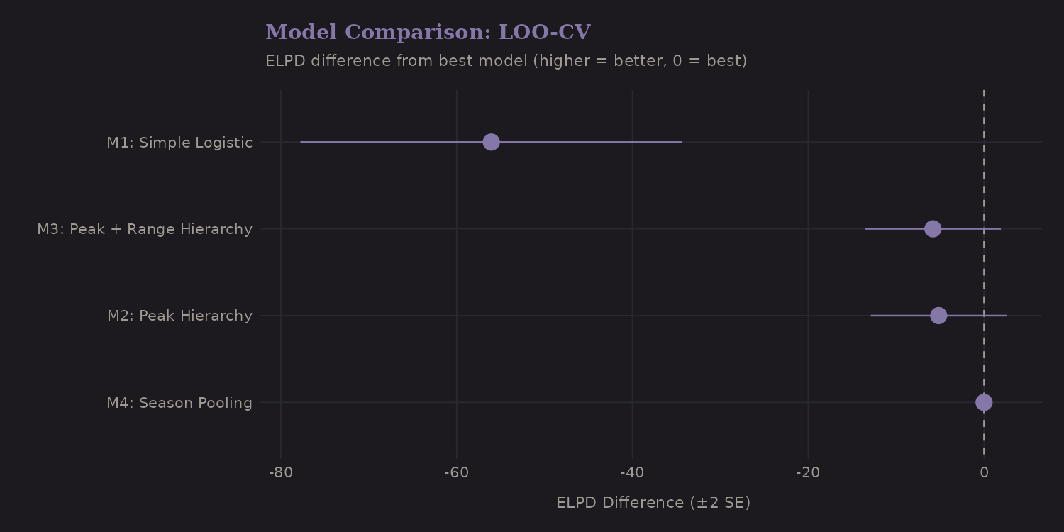
| Model | ELPD Diff | SE |
|---|---|---|
| M4: Season Pooling | 0.0 | 0.0 |
| M2: Peak Hierarchy | -5.2 | 3.9 |
| M3: Peak + Range Hierarchy | -5.8 | 3.9 |
| M1: Simple Logistic | -56.1 | 10.9 |
The hierarchical models (M2-M4) substantially outperform the simple model (ΔELPD = -56). Adding peak-level random effects captures important structure. The nested hierarchy (M3) and season-varying slopes (M4) provide marginal improvements—within standard error of each other.
Implementation detail: I enable moment matching for LOO when the fitted
model saved the required parameters; older fits without save_pars(all=TRUE)
fall back to standard LOO, so re-fit if you want fully stabilized estimates.
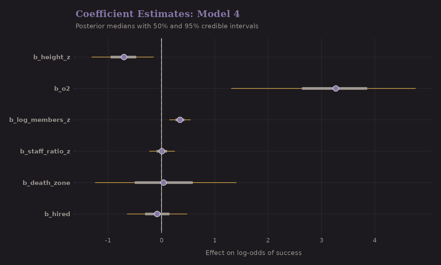
Fixed Effects
How do the coefficient estimates change across models?
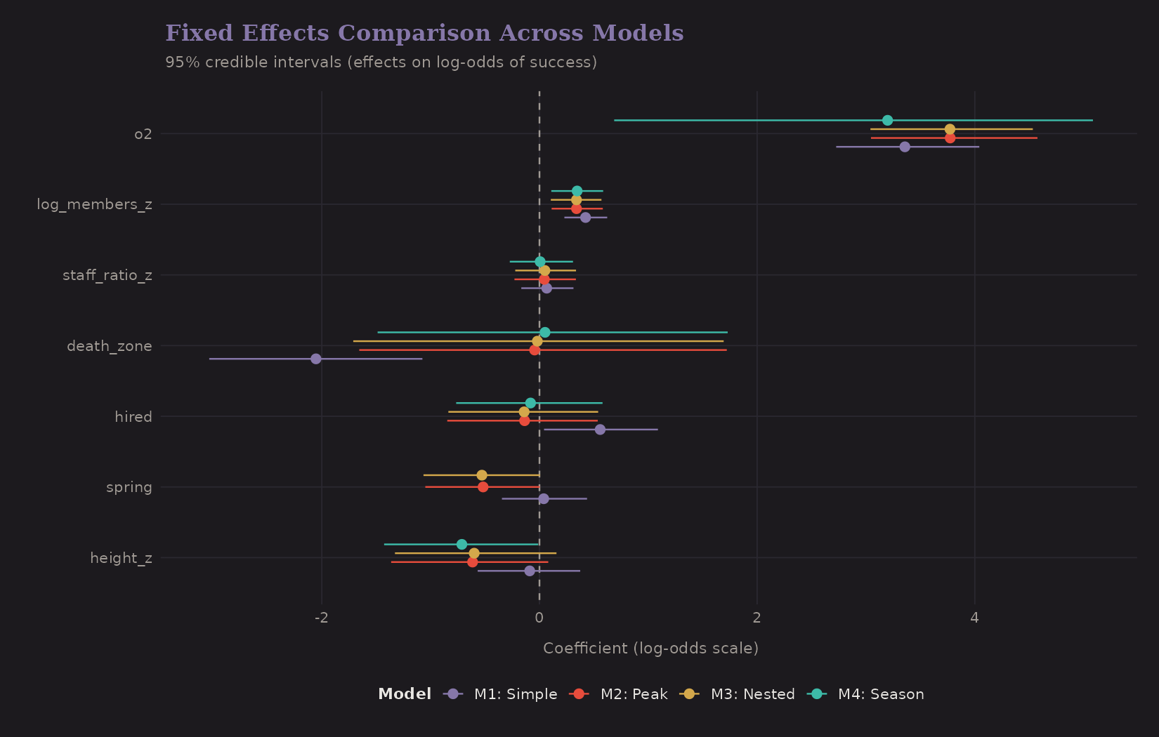
Key observations:
- Oxygen (o2): Effect size 3.77 (95% CI: 3.05 to 4.58) on log-odds scale. This translates to ~44× increase in odds of success—the dominant predictor.
- Height: -0.61 (95% CI: -1.36 to 0.08) per SD increase. Higher peaks have lower success even after controlling for oxygen.
- Death zone (8000m+) shows additional difficulty beyond continuous height.
- Effects are fairly stable across model specifications, which is reassuring.
The hierarchical models have slightly different point estimates because they account for clustering. When observations aren't independent, ignoring that structure biases standard errors (usually downward).
Peak Random Effects
Model 2 adds random intercepts for each peak (SD = 1.14). These capture unobserved peak-level factors: technical difficulty, weather patterns, infrastructure.
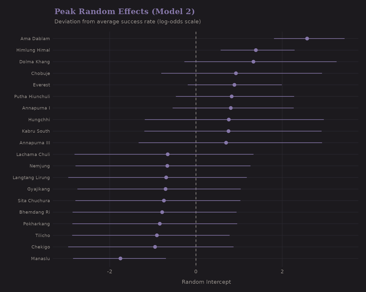
The extremes are interesting:
- Easy peaks (positive random effects): higher baseline success than average for their height
- Hard peaks (negative random effects): lower success even after accounting for measured predictors
This variation is what hierarchical models capture—the "unexplained" peak-level difficulty that remains after controlling for observables.
Variance Partition
Model 3 nests peaks within mountain ranges (Himals). How much variance occurs at each level?
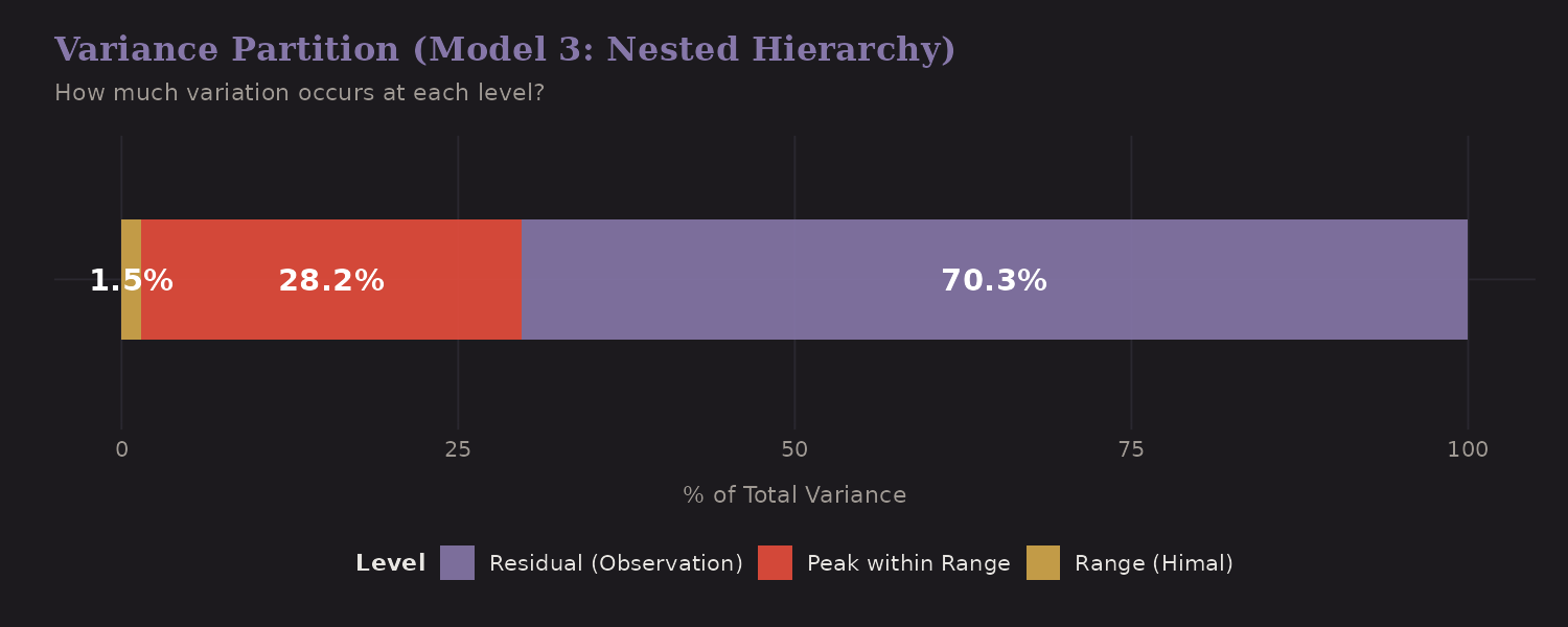
The variance decomposition:
| Level | Variance Share |
|---|---|
| Range (Himal) | 1.5% |
| Peak within Range | 28.2% |
| Residual (expedition) | 70.3% |
Most variance is at the observation level (expedition-specific), with meaningful peak-level variation (28%). The range level contributes little— peaks within the same range aren't dramatically more similar than peaks across ranges, once you control for height.
This has modeling implications: peak random effects matter; range random effects add complexity without much predictive gain.
Season-Varying Oxygen Effects
Does oxygen help equally in all seasons? Model 4 allows the O2 effect to vary by season:
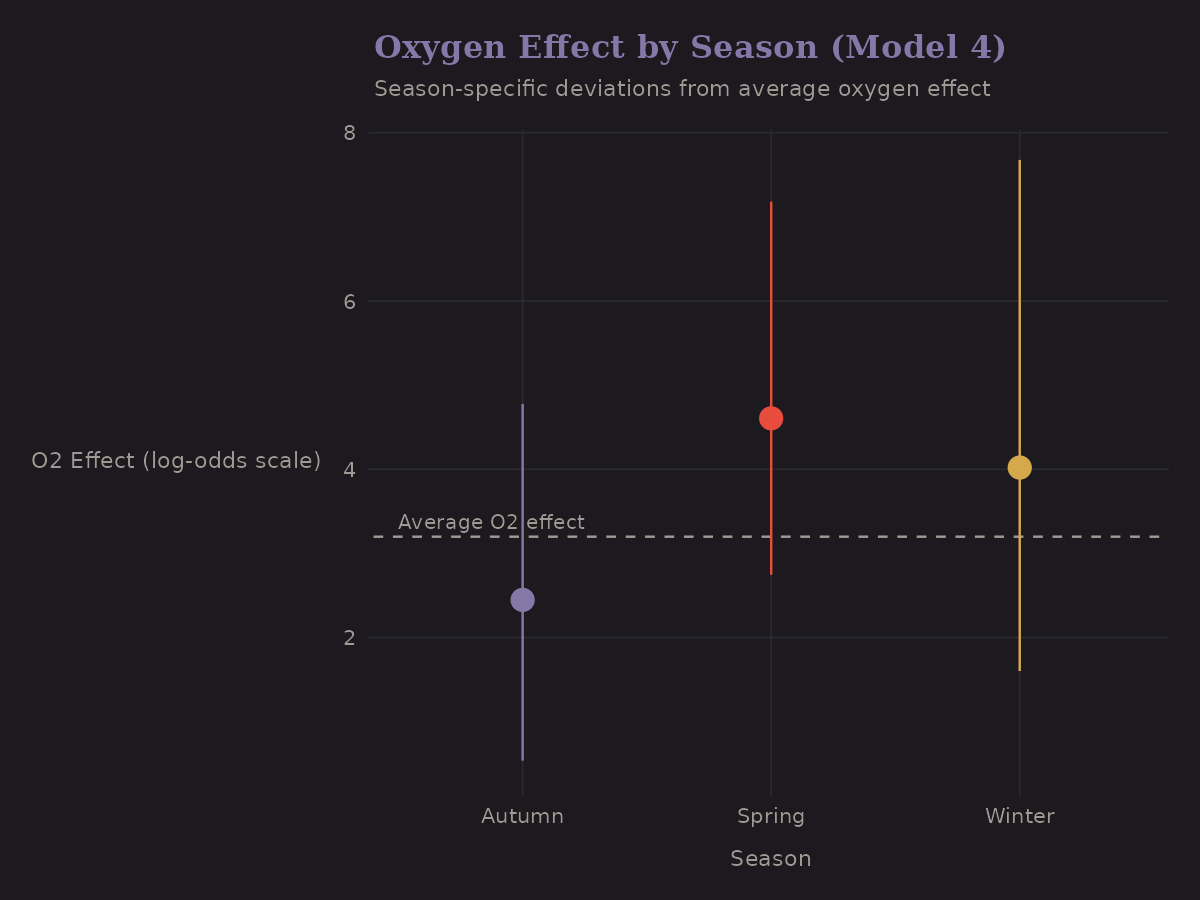
The differences are modest. Spring (the main climbing season) shows the expected oxygen benefit. Other seasons have wider uncertainty due to smaller samples.
This illustrates partial pooling in action—the season-specific estimates are shrunk toward the overall mean. If a season has few observations, its estimate won't stray far from average.
Posterior Predictive Check
Does the model generate data that looks like the observed data?
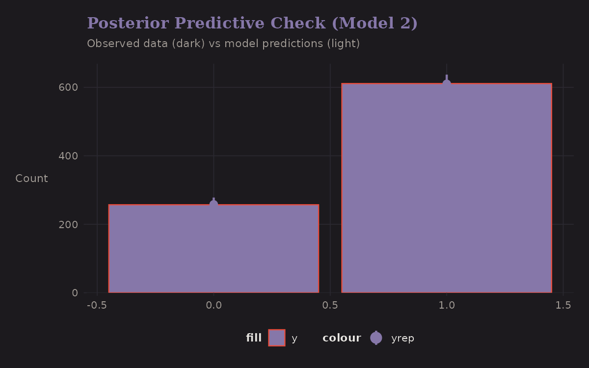
The predicted distribution matches the observed success/failure split reasonably well. This is a sanity check—if the model couldn't reproduce basic features of the data, something would be wrong.
Predicted Probabilities
What does the model predict for specific scenarios?
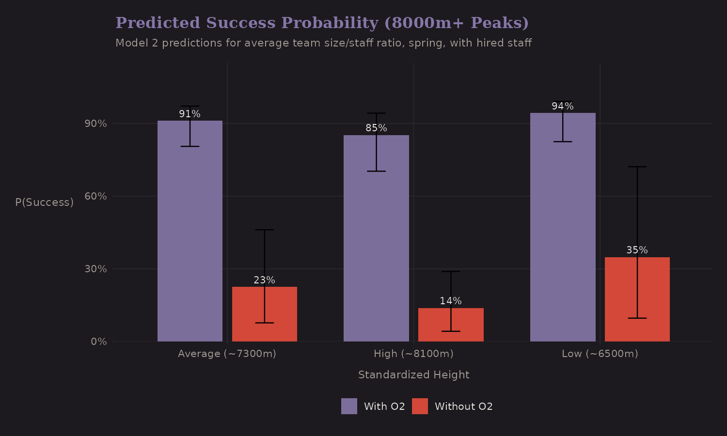
On 8000m+ peaks:
- With oxygen: ~85-90% success probability
- Without oxygen: ~15-25% success probability
The oxygen effect is substantial and robust. The error bars (credible intervals) capture posterior uncertainty—wider for scenarios with fewer observations in the training data.
MCMC Diagnostics
Bayesian models are only trustworthy if the MCMC sampler converged:
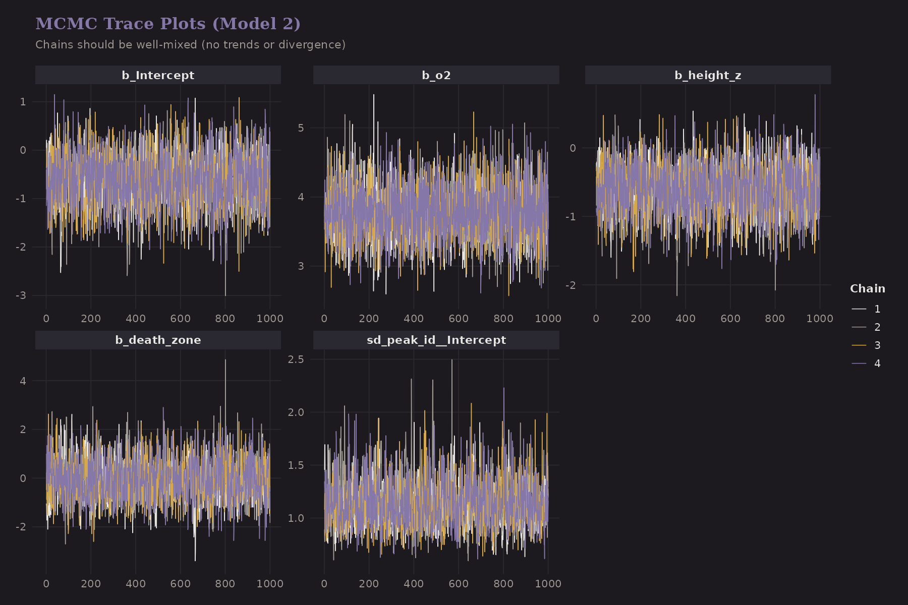
Good signs:
- Chains mix well (the "fuzzy caterpillar" pattern)
- No obvious trends or divergences
- All chains explore the same region
All models showed:
- R-hat < 1.01 for all parameters (indicating convergence)
- Effective sample sizes > 1000
- A couple of divergences in Model 4 at
adapt_delta = 0.95(fixable by raisingadapt_delta)
Survival Analysis
Model 5 takes a different perspective: instead of binary success/failure, model time to summit with censoring for expeditions that didn't make it.
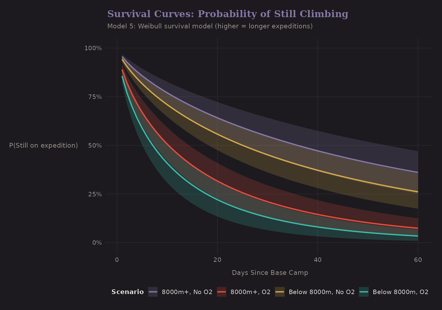
This is a Weibull survival model. The curves show the probability of still being on expedition (not yet summited) over time.
- 8000m+ without O2: Slowest, with many expeditions failing (censored) before summit
- Below 8000m with O2: Fastest progression to summit
Survival analysis is valuable when you care about when outcomes happen, not just whether they happen. For mountaineering, expedition duration affects cost, weather windows, and cumulative risk.
Oxygen Effect Heterogeneity
The average oxygen effect is strong, but does it vary by peak?
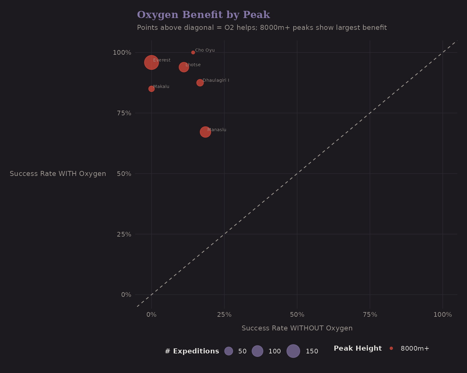
Each point is a peak (with at least 5 expeditions both with and without oxygen). Points above the diagonal show peaks where O2 helps; points on the diagonal show no benefit.
The 8000m+ peaks (red) show the largest oxygen benefit—which makes physiological sense. At extreme altitude, supplemental oxygen provides a much larger relative boost because baseline O2 availability is so low.
Bayesian Shrinkage
This is the core insight of hierarchical models:
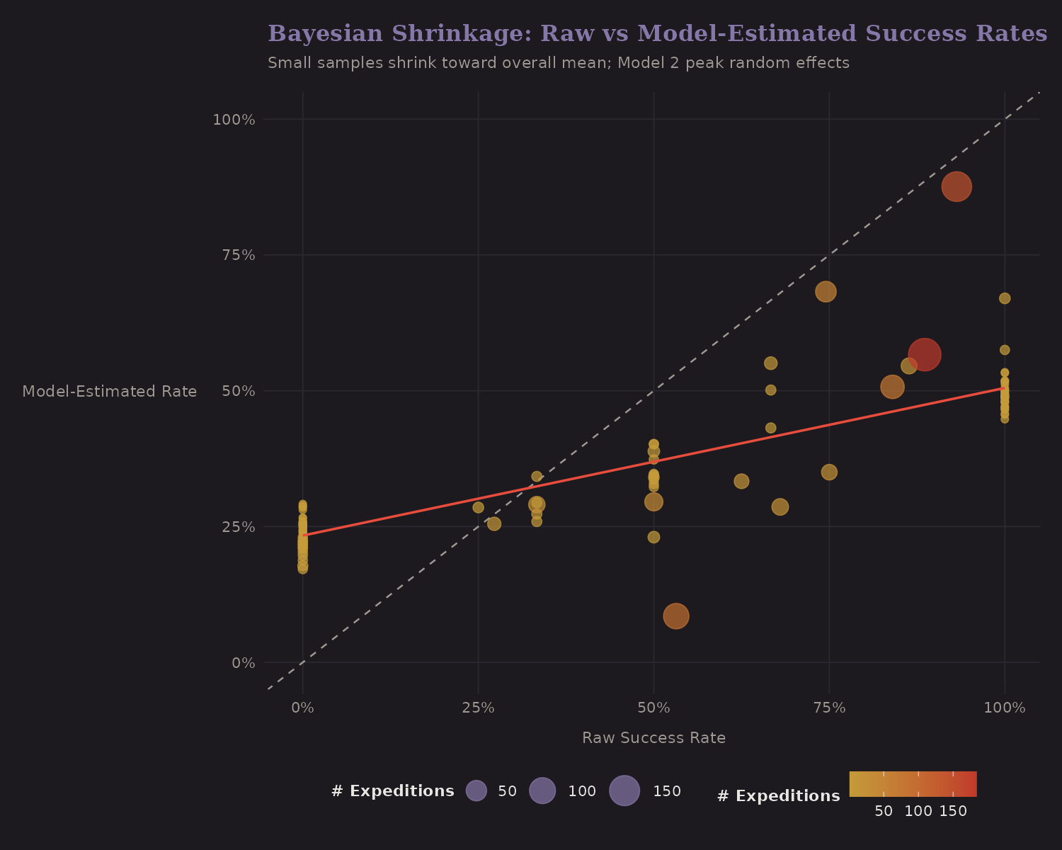
The x-axis shows raw success rates; the y-axis shows model-estimated rates.
- Large samples (big dots): Stay close to the diagonal (raw = estimated)
- Small samples (small dots): Pulled toward the overall mean
This is shrinkage—we don't fully trust extreme rates from small samples. A peak with 3 successful expeditions out of 3 doesn't really have a 100% true success rate. The hierarchical model recognizes this and adjusts.
Coefficient Summary
The best model's coefficients at a glance:
Positive effects on success:
- Oxygen use (dominant: +3.77 log-odds)
- Team size (log-scaled: +0.34 log-odds)
Negative effects:
- Height (standardized: -0.61 log-odds)
- Spring season (-0.52 log-odds, after controlling for O2)
Note: Spring appears negative because spring expeditions use oxygen more often. Once we control for oxygen, the direct season effect is slightly negative.
These effects are on the log-odds scale. To interpret magnitude, exponentiate: exp(2) ≈ 7.4x increase in odds for a 1-unit change in the predictor.
What I Learned
A few takeaways from Bayesian modeling:
-
Hierarchy matters. Adding peak random effects substantially improved fit. The data has structure; the model should respect it.
-
Oxygen is robust. The effect is large, positive, and stable across all model specifications. Whatever else changes, O2 helps.
-
Partial pooling works. Small-sample peaks get reasonable estimates via shrinkage. This is better than trusting raw rates or ignoring peak identity entirely.
-
Survival analysis adds perspective. Time-to-event modeling reveals patterns that binary outcomes miss.
-
Bayesian workflow scales. With
brmsand Stan, these models are easy to specify and diagnose. The computational cost is manageable.
Limitations
A few important caveats:
-
These are associations, not causal effects. The hierarchical models show that oxygen is associated with success conditional on peak effects, but this isn't causal identification.
-
Unmeasured climber skill remains a concern. The models control for team composition but not individual climber ability or experience.
-
Hierarchical structure helps but doesn't solve confounding. Peak random effects capture peak-level variation but don't address expedition-level confounders.
-
Temporal scope is limited. The 2020-2024 data may not generalize to earlier periods when climbing technology and practices differed.
The causal inference post addresses some of these limitations with propensity scores and sensitivity analysis.
What's Next
The models so far show association. Oxygen use is correlated with success, but is that causal? The next post explores this with Probabilistic Graphical Models—DAGs, Bayesian networks, and structural equation models with latent variables.
Code
The analysis used R with brms, bayesplot, and tidybayes. Key model
specification:
model2 <- brm(
  success ~ height_z + o2 + log_members_z + staff_ratio_z +
            death_zone + spring + hired + (1 | peak_id),
  data = model_data,
  family = bernoulli(link = "logit"),
  prior = c(
    prior(normal(0, 2.5), class = "Intercept"),
    prior(normal(0, 2.5), class = "b"),
    prior(exponential(1), class = "sd")
  ),
  chains = 4,
  iter = 2000,
  seed = 42
)
The (1 | peak_id) syntax adds random intercepts for each peak. The priors
are weakly informative—they allow the data to dominate while preventing
extreme estimates.